R E C – T E C

P R O F E S S I O N A L

PrtSc

I N S I D E R E C - T E C

Training Manual and Tutorial

George M. Bonnett, JD

REC-TEC LLC

P.O. BOX 561031

ROCKLEDGE, FLORIDA 32956-1031

321-271-6459

Copyright George M. Bonnett, JD 2018 All Rights Reserved

DISCLAIMER

The information contained in this manual is based to the best of REC-TEC LLC’s knowledge on viable although innovative practices in the investigation of incidents as applied to vehicular collisions. However, neither REC-TEC LLC nor the author assumes any liability in connection with the use of this material. Every acceptable procedure may not have been presented and some circumstances may require additional or substitute procedures. Also, statutes, ordinances and organizational policies differ widely and wherever these are in conflict with the information contained herein, the former should govern.

COPYRIGHT

Copyright © 2018 by George M. Bonnett, JD. All rights reserved. No part of this publication may be reproduced or transmitted in any form or by any means, electronic or mechanical, to include photocopying and recording, or by any information storage and retrieval system, without prior permission in writing from the author.

When Viewing This Document

Select View then Text Size or Zoom in your Browser (or the Zoom feature in the lower right corner of most Browsers) to change the way this manual appears on the screen.

TABLE OF CONTENTS (Underline indicates Hyperlink – Click Back Arrow in Browser/Cell Phone to Return)

This entire document was assembled using Microsoft Word, Screen Hunter 6 (free) and REC-TEC Platinum software. All screen shots were captured using REC-TEC Platinum Software, [Alt PrtSc], or Screen Hunter 6 for Screens with drop down or sub menus.

• Introduction
  
• Configuration
  
• Modules

• Upper Navigation Bar Features

• REC-TEC Menu
• Files
• Setup
• Edit
• Tools
• Vehicles
• Internet
• Help
• Manual
• Google
• License Name

• Lower Navigation Bar Features

• Capture Image
• Print Image
• Report Form
• Graphics
• Vehicle Specs
• Cycle Windows
• AutoLoad

• Time – Distance

• Module 1 – Acceleration-Deceleration (Rate/Factor)

• Module 2 – Acceleration Single Surface

• Module 3 – Deceleration Single Surface

• Motion Analysis Module – [Module 18]

• Module 4 – Multiple Vehicle

• Module 5 – Multiple Events

• Module 6 – Multiple Surfaces

• Module 7 – Time - Distance (Acc~Dec)

• Time - Distance (EDM) – [Module 53]

• Module 8 – Time - Distance – Omni

• Time - Distance – V-Trax Animation Module – [Module 54]

• Collision Avoidance

• Module 9 – Braking Maneuvers

• Module 10 – Collision Analysis

• Module 11 – Following Maneuvers

• Module 12 – Passing Maneuvers

• Separation Distance – [Module 59]

• Module 13 – Turning Maneuvers

• Fall – Vault

• Module 14 – Airborne

• Module 15 – Pedestrian Vaults

• Module 16 – Vault Slide Integration

• Yaw – Critical Speed

• Module 17 – Critical Speed of Curve – Yaw

• Module 18 – Motion Analysis

• Module 19 – Motorcycle Lean Angle

• Swerve and Recovery – [Module 3]

• Turning Maneuvers – [Module 13]

• Momentum

• Module 23 – 360 Digital Momentum

• Module 24 – 360 Linear Momentum

• Module 25 – 360 LM Omni & PDOF Lite (V1 and/or V2)

• Module 26 – Angular Momentum

• Module 27 – Low Speed Collisions

• Module 28 – Replaced by Module 25 (360 LM Omni)

• Energy - Damage Analysis

• Module 29 – Crash3 (Crush5 - DeltaV from Damage)
• Module 29A – Solving for Impact and Post-Impact Speeds in CRUSH
• Module 29B – Accuracy of Non-Equidistant “C” measurements
  
  
• Module 30 – Crush (Lite)

• Module 20 – Conservation

• Module 21 – Kinetic

• Module 22 – Energy > Break Fracture

• Pole > Narrow Object Impact – [Module 56]

• Module 31 – Reduced Mass (CEES)

• Module 32 – Stiffness Coefficients

• Energy – Crush (Motorcycle) – [Module 57]

• Miscellaneous

• Module 33 – Rotation Factor

• Module 34 – Speed – Hydroplane

• Module 35 – Speed – RPM

• Module 36 – Tangent Offset

• Module 37 – Weight Shift (3-Axis)

• Railroad Grade Crossings

• Module 38 – AASHTO/AREA Vertical Alignment

• Module 39 – AASHTO Sight Triangle

• Module 40 – Electronic Rail Circuits

• Module 41 – Combined Speed Formula

• Module 42 – Conversions

• Module 43 – Quadratic Solver

• Module 44 – Triangle Solver

• Module 45 – Statistical Range (Monte Carlo)

• Module 46 – Photogrammetry (2D)

• Heavy Truck

• Module 47 – DISC/S-CAM III/V Air Brake

• Module 48 – Load Check A (Tractor - Trailer)

• Module 49 – Load Check B (Straight Truck - Bus)

• Module 50 – Maximum Off-Tracking

• Module 51 – Rollover

• Module 52 – Weight & Balance

• Module 53 – Time - Distance (EDM)

• Module 54 – Time - Distance – V-Trax

• Module 55 – SMAC-RT

• Module 55B – New Procedures and Protocols in SMAC-RT

• Module 56 – Energy > Pole / Narrow Object Impact

• Module 57 – Energy – Crush (Motorcycle)

• Module 58 – Vectors (EDR – Momentum)

• Vectors and New Technology – An Alternative Approach

• Module 58B – Vectors (Inline Momentum)

• Module 59 – Collision Avoidance – Separation Distance

• Module 66 – Traffic Engineering – School Bus Stop

• Module 67 - Traffic Engineering – Work Zone (MUTCD)

• Module 68 - DrawPad

• Module 60: Drive3 Manual – Overview

• Module 61: Drive3 – Path Intrusion (Front)

• Module 62: Drive3 – Path Intrusion (Side)

• Module 63: Drive3 – Traffic Signal Response

• Module 64: Drive3 – Vehicle Changing Lanes

• Module 65: Drive3 – Vehicle Following

• Appendix A – EFFECT OF GRADE ON KINETIC FRICTION

INTRODUCTION:

(Table of Contents)

This workbook will cover all of the modules in the Platinum version of REC-TEC. Problems will be shown using the Imperial system of measurement. REC-TEC can work in any Imperial/Metric (or hybrid) system and can be switched between systems at any time. It will assist in becoming familiar with the various modules, and show how the program can solve very different, difficult, and complex problems. The workbook uses a step-by-step approach to REC-TEC accident reconstruction. It is not intended to teach the basics of accident reconstruction, but to assist the accident reconstructionist in solving problems using REC-TEC.

Fundamentals of Traffic Crash Reconstruction, Volume 2 of the Traffic Crash Reconstruction Series by John Daily, Nathan Shigemura, and Jeremy Daily, published by IPTM, is highly recommended as a basic tool for learning the science and art of accident reconstruction.

Figure 1

Figure 1 shows the new Help (F1) & Manual/Tutorial (F5) selections on the upper navigation bar (October 2015). Both are 'module sensitive' in REC-TEC Platinum.

REC-TEC BASICS

REC-TEC takes a modular approach to accident reconstruction problem solving, just as reconstructionists have always done. Each problem is broken down into solvable components:

· Determine the primary objective of the investigation.

· Break the overall problem down into solvable components.

· Combine the individual answers into a unified solution to the problem.

With these steps in mind, we will begin to solve problems using REC-TEC.

It is suggested that you work the problems on your computer as we go through them in the workbook in order to receive the maximum benefit from this workbook.

Navigating the Program

Before we begin to work problems, it may be beneficial to take an in depth look at the main screen and take a tour of the many features to get a better understanding of the functionality of the program. In addition to the new module sensitive selections on the upper navigation bar, the F1 – F5 keys also work from the Main screen. The F5 Key will call this document from the REC-TEC web site.

NEW ***** GLOBAL ENHANCED GRAPHICS (May 2014 Upgrade)

Figure A

Figure A displays the new "eGraphics" button on the Lower Navigation Bar. When the button shows eGraphics the new graphics upgrades will replace the original graphics functions. Graphics and eGraphics are toggled using the selection "Toggle Enhanced Graphics (Platinum)" on the Down Arrow button to the right of the Graphics/eGraphics button as seen in Figure B.

Figure B

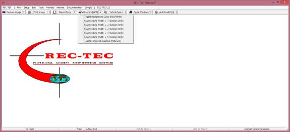
eGraphics consist of crosshairs that follow the cursor on selected graphics screens throughout the program. Two or more blocks will also appear with Time, Distance, Speed, or Lateral Distance matching the crosshair position. The crosshair position and data blocks can be "frozen" or "unfrozen" using the [Ctrl] key. This allows the cursor to be moved for other purposes such as clicking on the Report button to place the image in the report, or drawing on the image using the right mouse button as in original Graphics.

Modules with the enhanced graphics include:

· Collision Avoidance Following Maneuvers

· Collision Avoidance Turning Maneuvers

· Time Distance Acceleration

· Time Distance Deceleration

· Time Distance Multiple Vehicles

· Time Distance Omni

· Time Distance (EDM)

eGraphics is a Platinum Option only upgrade that also includes a unique new feature in the Time Distance (EDM) module. When the crosshairs are on the TD-EDM graphics, clicking on the left mouse button will immediately capture the point on both curves where the vertical crosshair is located and will place the corresponding Time, Distance, and Speed in the center data blocks below the graphics.

As before, the Data blocks below the Graphics screen can still be used to find and position a set of crosshairs on the Graphics corresponding to a Time, Distance or Speed. The new eGraphics permits using the vertical crosshair to select a position on the either curve and get the corresponding Time, Distance, and Speed information.

CONFIGURATION

(Table of Contents)

Figure 2

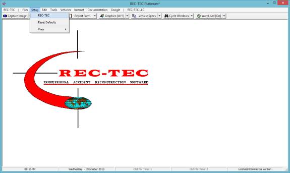
On the upper navigation bar of the main screen, select Setup > REC-TEC (Figure 2) to call up the Configuration screen (Figure 3). All problems will assume the following configuration unless otherwise specified:

Figure 3

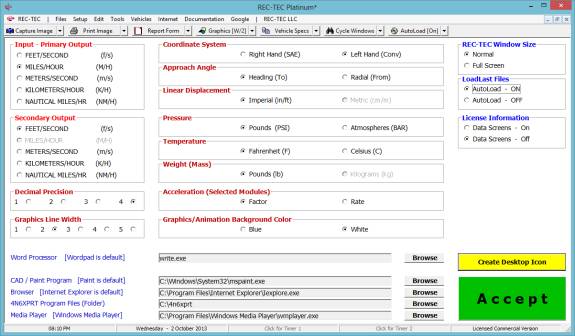
The preferences selected using the Configuration screen (Figure 3) will be set every time the program is started. This screen may be called at any time to change the preferences set at program start. Temporary changes can be made in the various modules or by using the Graphics Icon (or drop-down) on the main screen.

The configuration screen will set the basic input/output displays throughout the program as well as which additional programs REC-TEC will call (word processors, drawing packages, etc.). The F1 help files may be translated into many languages. Use the F7 key to pull up the HTML file from the website and right clicking on the English version in order to use one of the many Translation Accelerators now available.

Many display options can be set here as the default, but can be changed temporarily from the Graphics icon on the lower navigation bar.

Modules

(Table of Contents)

REC-TEC consists of various modules that, by treating your computer as a computer instead of a calculator, compute the answers for the maneuver, not just a single formula. Most modules offer iteration and graphics. Many offer animation and finite difference analysis. These tools will assist the professional in analyzing the problem and help provide confidence in the solutions. Many of the modules will integrate with other modules, providing additional analysis and support.

Upper Navigation Bar

(Table of Contents)

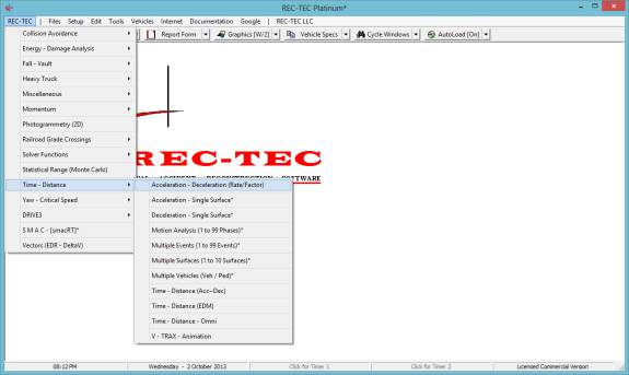
Opening a module – At the REC-TEC pull down menu (upper navigation bar – left side), select Time - Distance then Acceleration - Deceleration (Rate/Factor) from the submenu (Figure 4).

Figure 4

Note: Modules followed by an asterisk are capable of generating an animation text file. These files can be imported into third-party animation software capable of creating high-resolution animation using the X, Y, and Z positions for each time key frame computed by REC-TEC. A list of these modules and what is required is in the Manual > Overview Help file.

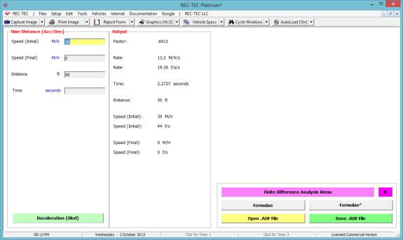
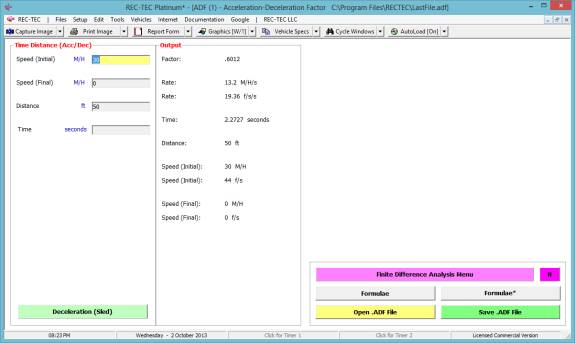
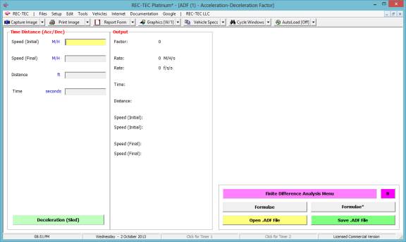
Click on Acceleration - Deceleration (Rate/Factor) and the Time - Distance Acceleration - Deceleration screen appears (Figure 5).

Figure 5

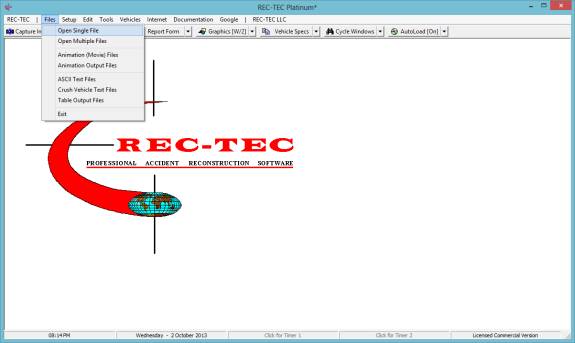
As an alternative, a file (or multiple files) can be selected from the upper navigation bar Files > Open Single File (Figure 6) or Files > Open Multiple Files.

Figure 6

This will call up a box showing all of the files in the Folder selected.

Figure 7

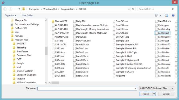
Clicking on Open will call up the Module and automatically open the file in the appropriate module (Figure 8).

Figure 8

If Open Multiple Files is selected, the user may open multiple files in one or more modules. To end this process, click on the Cancel button in the file display box.

Notice in Figure 8, on the lower navigation bar on the right hand side the icon labeled AutoLoad. In Figure 8, AutoLoad is turned off (AutoLoad[Off]). When a module is exited, or the program is exited, all modules save their current data to a file named “Lastfile” with the appropriate extension for the particular module.

Caution – if multiple copies of the same module are opened with different files, be sure to save the data as “named” files as the last module to close will overwrite the other “Lastfile” in identical modules.

Files – Opening and Saving Files

Almost every module allows saving the data to a file that can be re-opened later, redisplaying the original computations. Each of these text files carries an extension (.???) unique to a particular module. When a module is closed, the data (or lack of data) in that module is automatically saved as Lastfile.(ext). If AutoLoad is set to [On], the file for the module will open using this Lastfile.(ext) unless the module is opened by selecting a particular named file.

Once a module is open, a file can be opened at any time using the Open .EXT File button. The Save .EXT File button will save the data with a user selected name.

Other Files options are available which call up text files produced by various modules for third party animations. Many popular movie (animation) formats can also be called up using the Files menu.

Setup

The submenu > REC-TEC calls up the Configuration screen, which can be viewed or modified.

The submenu > Reset Defaults calls up the Configuration screen with the default settings, which can be viewed or modified.

The (Figure 9) submenu > View permits the user to independently view or hide the lower (Icon) navigation bar and the Status bar at the bottom of the screen.

Figure 9

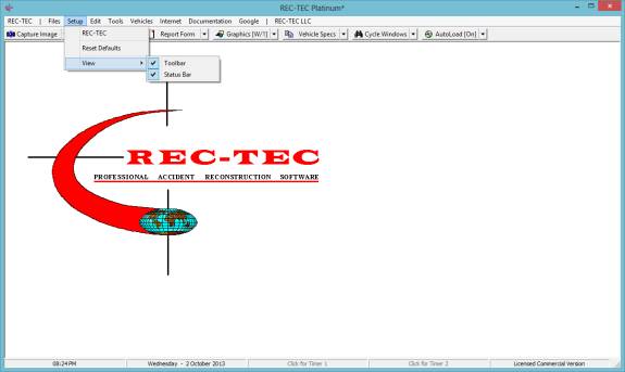
Figure 10 (Removed in 2015) - Functions Duplicated on Lower Navigation Bar

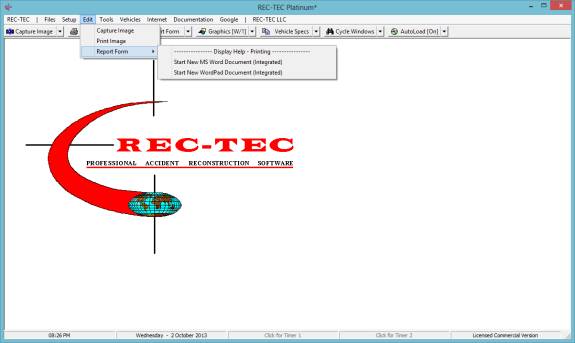
Edit (Figure 10) - (Functions duplicated on Lower Navigation Bar)

Figure 11

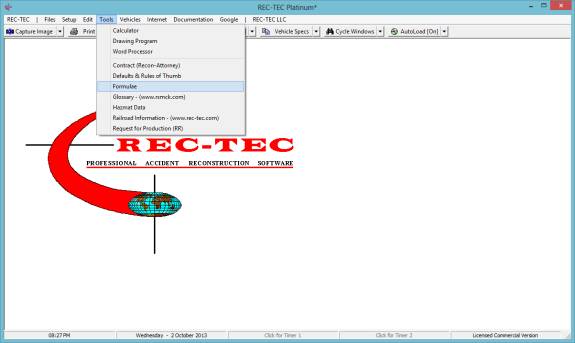
Tools (Figure 11)

· Submenu > Calculator: Windows Calculator (Switches between Normal and Scientific).

· Submenu > Drawing Program: Set on Configuration screen.

· Submenu > Word Processor: Set on Configuration screen.

· Submenu > Contract (Recon-Attorney): Sample contract.

· Submenu > Defaults & Rules of Thumb: Collection of values.

· Submenu > Formulae: Formulae used in program (two formats).

· Submenu > Glossary – (rsmck.com): Useful AR glossary.

· Submenu > Hazmat Data: Hazmat information.

· Submenu > Railroad Information (rec-tec.com): Useful Railroad information.

· Submenu > Request for Production (RR): Sample document (Railroad).

Figure 12

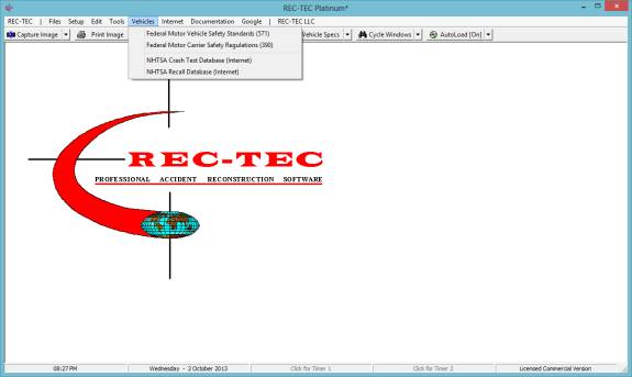
Vehicles (Figure 12)

· Federal Motor Vehicle Safety Standards (571)

· Federal Motor Carrier Safety Regulations (590)

· NHTSA Crash Database (Internet)

· NHTSA Recall Database (Internet)

Figure 13

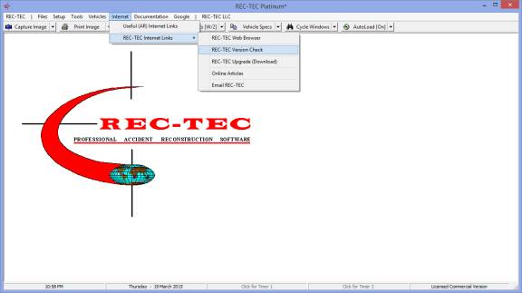
Internet

• Useful AR Internet Links (Figure 14)
• REC-TEC Internet Links
• REC-TEC Web Browser
• REC-TEC Version Check (Removed 2015 - Click on License Name)
• REC-TEC Upgrade (Download)
• Online Articles
• Email REC-TEC

Figure 14

Documentation (Figure 15)

• REC-TEC - Email Information for License
• All F1 Key (Help).PDF Files
• [F1] key Program Overview or Help
• [F2] key Finite Difference Analysis Overview
• [F3] key Animation Overview
• [F4] key Module Overview
• [F5] key Inside REC-TEC (www.rec-tec.com)
• [F6] key Same as [F1] key
• [F7] key Same as [F1] key (www.rec-tec.com)
• [F8] key Inside REC-TEC (PDF)
• [F9] key REC-TEC Startup Guide (PDF)
• [F10] key REC-TEC Version Check (www.rec-tec.com)
• About Coordinate Systems (Diagram of Coordinate Systems)
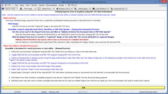
• Printing Reports and Graphics (Figure 16)

Figure 15

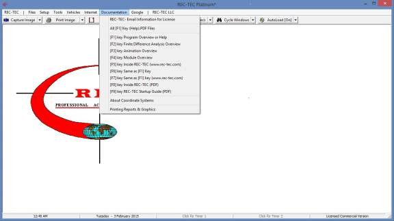
Figure 16

Google

· Calls Google for Answers to many AR/Other questions

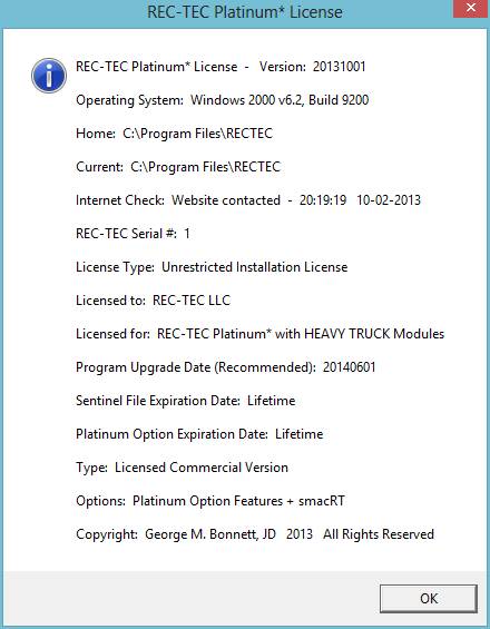
Name

· REC-TEC License (Figure 17)

Figure 17

Radio Button Functions

To the right of certain (Primary Output) Speeds in selected modules there is a “Radio Button” that will transfer the value of the Speed to the “Windows Clipboard” for transfer into other modules within REC-TEC or anywhere else the user may select using the Paste option after Right Clicking on the Mouse. This option appears on the following modules:

Time Distance Multiple Surfaces (Initial Speed)

Fall-Vault Airborne

Vault-Slide Integration

Yaw-Critical Speed of a Curve

Kinetic Energy

360 Linear Momentum (Impact Speeds)

At every entry point in the program calling for an Acceleration/Deceleration Factor, there is a small round “Radio Button.” Clicking the Radio Button will cause the Acceleration/Deceleration Factor module to appear. Computations can be made for timed or measured vehicle tests or for Drag Sled Pull weight divided by Sled weight. The user may then transfer the result of the computation and Exit the module or Exit the module without transferring a value.

Lower Navigation Bar (Icons and dropdown menus) – See Figure 1

(Table of Contents)

· Capture Image – Captures REC-TEC Image on Clipboard

o Capture Entire Screen

o Capture REC-TEC

o Capture REC-TEC (Active Form)

o Capture Active Window (time delayed capture)

o Display Captured Image (Displayed on REC-TEC Form)

o Clear Current Image

· Print Image – Prints REC-TEC image to default printer

· Report Form – Sets link to Word/WordPad/Adobe printer driver

o Display Help – Printing

o Initiate Document Link with Word (Integrated)

o Initiate Document Link with WordPad (Integrated)

o Activate PDF (Adobe) Document Spooler

o Copy Image to Report

o Close Document (Spooler to PDF Document)

· Graphics – Toggles Graphics background color

o Toggles Background Color (Blue/White)

o Graphics Line Width = 1 (Session only)

o Graphics Line Width = 2 (Session only)

o Graphics Line Width = 3 (Session only)

o Graphics Line Width = 4 (Session only)

o Graphics Line Width = 5 (Session only)

· Vehicle Specs – Calls AutoStats Lite from 4N6XPRT Systems

o List of 4N6XPRT Vehicle Specs programs installed on computer (if any)

o Canadian Vehicle Specs (Windows Version)

o Sisters and Clones

o Motorcycle Specs (Internet)

· Cycle Windows – Cycles (multiple) modules to foreground

o Cascade

o Tile Horizontally

o Tile Vertically

o Arrange (Icons)

o Minimize All

o Restore All

o Close All

· AutoLoad – Toggles AutoLoad[On/Off]

o Save Change

o AutoLoad – ON

o AutoLoad – Off

Module 1: Time - Distance – Acceleration-Deceleration (Rate/Factor)

(Table of Contents)

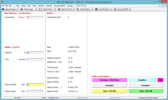
Overview: This module computes Acceleration/Deceleration factors and rates based on supplied information.

At the REC-TEC pull down menu, select Time - Distance > Acceleration-Deceleration (Rate/Factor) and the Time - Distance - Acceleration-Deceleration (Rate/Factor) screen appears (Figure 18).

Figure 18

Input Data

This module has four data inputs (No “required” inputs)

1. Initial Speed
2. Final Speed
3. Distance
4. Time

Two or three inputs are required to generate a solution.

· If Distance and Time inputs are used, the module will compute a solution. If a Speed input is added, the module solves for the unknown speed input.

· If a Distance and a Speed input greater than zero is used, the module will compute a solution. If Time or a second Speed input is added, the module will solve for the remaining unknown.

· If two Speed inputs are used, either Time, or Distance is required. The module will solve for the remaining unknown.

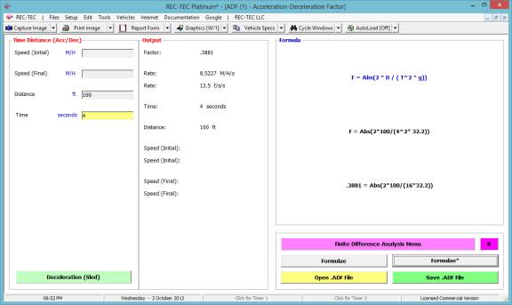
Example 1: A vehicle accelerates at a uniform rate traveling 100 feet in four seconds.

1. What is the acceleration factor?

2. What is the acceleration rate?

3. What is the final speed? Is there a way to determine the final speed with the information given?

Figure 19

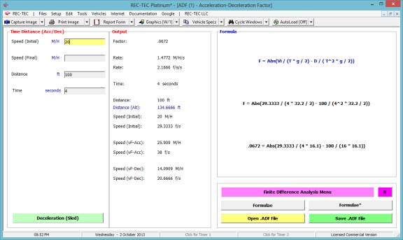
Example 2: A vehicle accelerates from 20 M/H at a uniform rate traveling 100 feet in three seconds.

4. What is the acceleration factor?

5. What is the acceleration rate?

6. What is the final speed?

Figure 20

Example 3: A vehicle decelerates to a stop at a uniform rate traveling 100 feet in three seconds.

7. What is the deceleration factor?

8. What is the deceleration rate?

9. What is the initial speed?

Figure 21

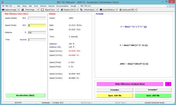
Figure 22

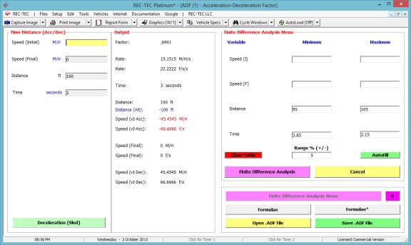
Figure 22 shows the Finite Difference Analysis menu for the Acceleration/Deceleration factor.

Figure 23

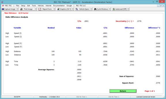
Figure 23 shows the results of the Finite Difference Analysis. This analysis is for the Acceleration (or Deceleration) factor only. It does not include the speeds unless they are part of the computation.

Iteration and Finite Difference Analysis

Iteration (table generation) is available in all versions of REC-TEC and is almost self-explanatory. It will be demonstrated in the Time - Distance Single Surface Deceleration, 360 Linear Momentum, S-CAM Air Brake and other modules that may represent unique variations on the basic iteration model.

Finite Difference Analysis (FDA), which computes an “Uncertainty Level” based on a specific range of the variables within a formula, is restricted to the Platinum Version of the program. A general explanation of the principles of FDA is called up by using the F2 key from any module offering FDA. FDA will be demonstrated in the 360 Linear Momentum, S-CAM Air Brake and other modules that may represent unique variations on the basic FDA model.

SAE paper 2003-01-0489 Evaluating Uncertainty in Accident Reconstruction with Finite Differences by Wade Bartlett and Al Fonda compares Finite Difference Analysis with the “Monte Carlo” type of computations done by various high-powered statistics programs on the market. For the same given ranges of the variables involved, the answers are identical.

Example 4: A 45-pound drag sled has a pull weight of 33 pounds.

Select Deceleration (Sled) – this selection is made from the screen shown in Figure 21.

10. What is the deceleration factor?

11. What is the deceleration rate?

Figure 24

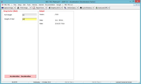
Figure (24B)

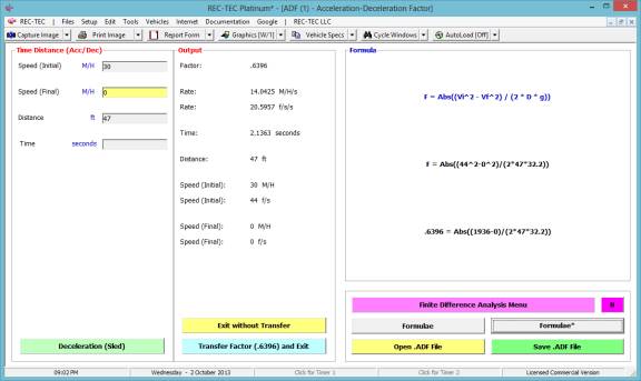
Figure (24B) shows the screen, as it would appear if it were called up using the new “Radio Button” feature already described above. The “factor” can be transferred automatically to the input on the calling module or this page can be exited without transferring.

Module 2: Time - Distance – Acceleration Single Surface

(Table of Contents)

Overview: This module computes detailed information on the Speed, Distance and Time of a single acceleration event.

At the REC-TEC pull down menu, select Time - Distance > Acceleration - Single Surface and the Time - Distance - Acceleration screen appears (Figure 25).

Figure 25

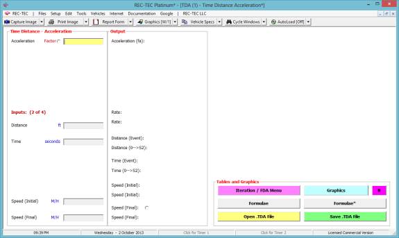
Required Input Data:

Acceleration Factor (fa): The percentage of gravity used to accelerate the vehicle. The acceleration factor is entered into the program as a decimal value representing a percentage of gravity available to accelerate the vehicle.

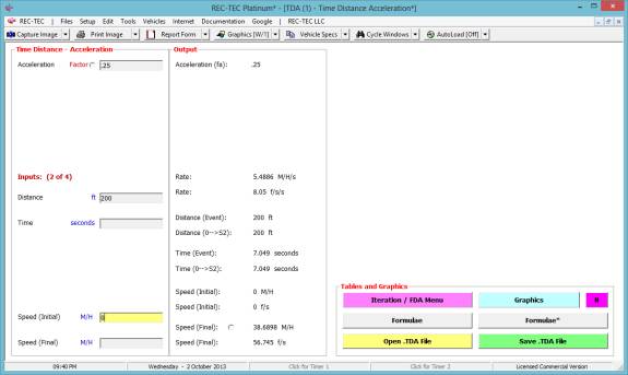
Example 1: The vehicle has an average acceleration factor of .25 “g” during the maneuver.

1. How fast was the vehicle traveling at the end of the acceleration if it started from a full stop and accelerated for 200 feet?

2. How long did the acceleration take?

Solution: Enter into the module the required data:

1. Acceleration Factor (.25)
2. Initial Speed (0)
3. Distance (200)

With this information, the final speed is computed at 38.6898 M/H (question # 1) and a time of 7.049 seconds to accelerate from a full stop (question # 2) as illustrated in Figure 26.

Figure 26

Example 2:

3. How fast was the vehicle traveling at the end of the acceleration if it started from 20 M/H and accelerated for 200 feet?

4. How long did the acceleration take?

Figure 27

With this information, the final speed is computed at 43.5534 M/H (question # 3) and a time of 4.2913 seconds to accelerate from 20 M/H (question # 4) as illustrated in Figure 27.

Example 3:

5. How fast was the vehicle traveling at the start of the acceleration if it accelerated for 200 feet to a final speed of 60?

6. How long did the acceleration for the 200 ft. take?

7. How long did the acceleration take if it was from a full stop to 60 M//H?

8. What was the distance covered in Question 7?

Figure 28

With this information, the initial speed is computed at 45.8595 M/H (question # 5) and a time of 2.5763 seconds to accelerate for 200 ft. to a final speed of 60 M/H (question # 6) as illustrated in Figure 28.

The time from full stop to 60 M/H is computed to be 10.9316 seconds (question # 7) and the total distance is 480.9937 feet (question # 8) as illustrated in Figure 28.

Iteration and Finite Difference Analysis

Iteration (table generation) is available in all versions of REC-TEC and is almost self-explanatory in nature, it will be demonstrated in the Time - Distance Single Surface Deceleration, 360 Linear Momentum and the S-CAM Air Brake modules, as they each represent unique variations on the basic iteration model.

Finite Difference Analysis (FDA), which computes an “Uncertainty Level” based on a specific range of the variables within a formula, is restricted to the Platinum Version of the program. A general explanation of the principles of FDA is called up by using the F2 key from any module offering FDA. FDA will be demonstrated in the 360 Linear Momentum and the S-CAM Air Brake modules, as they each represent unique variations on the basic model demonstrated in the Time - Distance Single Surface Deceleration, module.

Module 3: Time - Distance – Deceleration Single Surface

(Table of Contents) (Table of Contents)

Overview: This module computes detailed information on the Speed, Distance and Time of a single deceleration event. If lateral information is input, the module also computes detailed swerve and swerve-and-return data.

At the REC-TEC pull down menu, select Time - Distance > Deceleration - Single Surface and the Time - Distance - Deceleration screen appears (Figure 29).

Figure 29

Required Input Data

Coefficient of Friction – “Mu”: The coefficient of friction is defined as the percentage of gravity developed at the tire-road interface for acceleration (deceleration). The coefficient of friction is entered into the program as a decimal value representing a percentage of gravity available to decelerate the vehicle.

Grade – Grade is the rise or fall of the roadway. It is either a negative downhill grade or a positive uphill grade and is dependant upon your direction of travel. You may often hear it referred to as the “slope” of the road. Grade is determined by the ratio of the rise of the roadway divided by the run or length of the measurement. It is the tangent of the angle.

The Grade of the roadway is entered into the program using a positive uphill or negative downhill decimal value. If no entry is made, the module treats the grade as zero.

Braking Percentage – the braking efficiency of the vehicle is a determination of how much of the entire weight of the vehicle is being overcome by the brake force generated at the wheels. As the vertical weight at each brake point increases, a limit is reached when the components of the brake assembly will no longer generate enough force to overcome the rotational torque of the wheel. This limit is dependant upon the vertical weight component on each wheel and the overall mechanical condition of the brake components.

Braking efficiency is entered in the program as a whole number percent value as opposed to a decimal value. Full braking on all wheels is entered as 100 (100%).

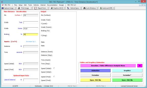
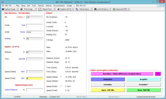
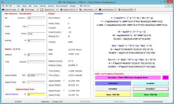
Example 1: A vehicle skids 47 feet before striking a pedestrian crossing the roadway. It continued for an additional 20 feet before coming to a complete stop. An accelerometer was used to conduct skid tests and it was determined that the coefficient of friction of the roadway was 0.73. The grade at the accident site was a negative 2% and the crash vehicle had a overall braking efficiency of 70%.

1. How fast was the vehicle traveling at impact with the pedestrian?
2. How fast was the vehicle traveling when the driver first applied the brakes?
3. How long did it take the vehicle to skid to a stop?
4. How long did it take the vehicle to skid to impact with the pedestrian?
5. If the vehicle would have had 100% braking, would the collision with pedestrian occurred?

Solving the problem

Step 1: Determine from the problem what data is available for input into the module

• Distance of skid to impact: 47 feet

• Distance of skid after impact: 20 feet

• Total distance of skid: 67 feet

• Ending speed/velocity: 0 mph

• Coefficient of Friction: 0.73

• Grade: -0.02

• Braking efficiency: 70 %

• Optimum braking efficiency – 100%

Step 2: Enter into the module the required data:

• Coefficient of Friction

• Grade at crash site

• Braking efficiency

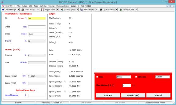
Figure 30

Solution: This module requires two of the following four variables to reach a solution.

1. The beginning speed/velocity,
2. The ending speed/velocity,
3. The distance of skid,
4. The time of the skid.

From the information given, we have two known values that can be used to determine a solution and answer the general questions that may be raised during the normal course of our reconstruction. We know that the vehicle skids to a stop and therefore have an ending speed/velocity of 0 mph. We also know that the vehicle skids 47 feet pre-impact, 20 feet post-impact for a total skid distance of 67 feet. Using these two known values we can answer Question 2 and Question 3 of our problem.

Step 3: Enter 67 feet as the distance of skid to a stop and 0 miles per hour as the final speed of the vehicle.

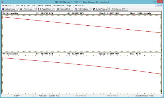
With this information, the initial speed is computed at 31.3795 M/H (question # 2) and a time of 2.9115 seconds to skid to a full stop (question # 3) as illustrated in Figure 31.

Figure 31

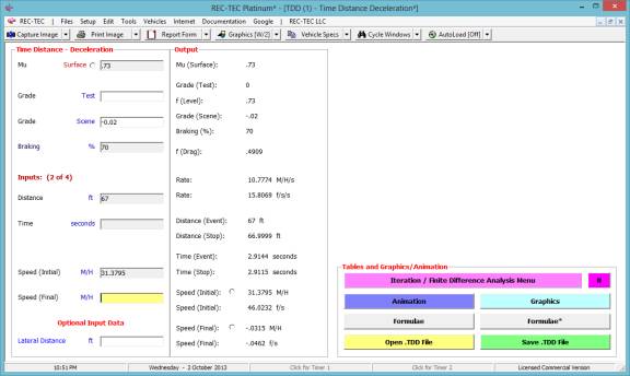
Question #2 concerning the initial speed of the vehicle (31.3795 M/H) and question #3 about the time to decelerate to a stop (2.9115 seconds), have now been answered. The program has computed the speed at the start of the deceleration as 31.3795 M/H and while the reconstructionist would never use a four decimal point answer for the initial speed in testimony, this is our computed initial speed for further computations.

Enter the initial speed/velocity of 31.3795 M/H and the distance to the pedestrian of 47 ft as known values.

Figure 32

The program has now computed the answers to question # 1 (17.1444 M/H) and question # 4 (1.3208 seconds). The only question left is #5.

By entering 100 for the percent of braking, we find that a distance of 46.3337 feet is required to come to a full stop and that at 47 feet the vehicle would be traveling at –3.7629 M/H. The collision with the pedestrian would not have occurred.

Figure 33

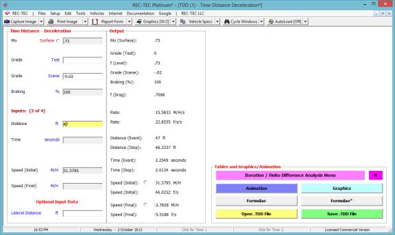
Figure 34

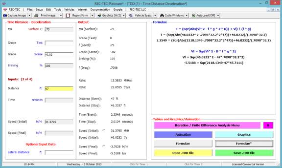
The Formulae* button will bring up a screen showing the formulae required to compute the two missing variables (Figure 34).

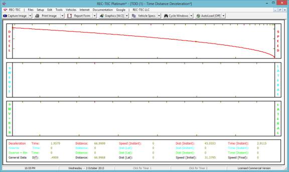
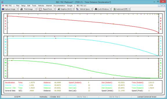
The Graphics button will show the Speed versus Time and Speed versus Distance graphs.

In Figure 35, the curves are shown for 70% braking.

Figure 35

The Animation button will display the deceleration curve for the Time or Distance entered in the blocks in Figure 36. Entering a number greater than 1 will display the animation in slow motion.

Figure 36

Notice that in Figure 37 the 47 foot mark is shown as a small circle on the curve.

Figure 37

This module has an optional input – Lateral Distance. This distance could be the width of a lane or the distance the vehicle must move laterally in order to miss the object. This module computes the lateral movement based on the full friction value of the coefficient of friction. The following figures will show a Lateral Distance of 12 feet. The additional data the module is able to compute is displayed in Figure 38 and described more fully in the Help file available by using the F1 key while in this module.

Figure 38

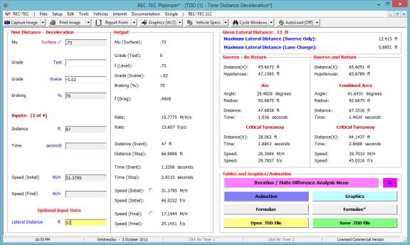
Figure 39

The Formulae* screen now displays the basic formulae and computations for the distances required for the Swerve and Swerve & Recover Distance computations as shown in Figure 39.

Swerve-No Return shows what would happen if the vehicle were placed in a maximum rate change of direction using the coefficient of friction (modified for grade). This is the same as using a .71 G turn using the numbers in this example. This would allow the vehicle's center of mass (or any given point of reference) to pass 12 feet laterally from the initial path of travel. This would NOT have the vehicle headed on a parallel path; it would be headed in a different direction (like off the road and into the boonies?). If the vehicle were brought back to a parallel path, the distance and time would be doubled as would the total lateral distance.

Swerve and Return shows what would happen if the vehicle were placed in a maximum rate change of direction using the coefficient of friction (modified for grade) with an immediate change to a maximum rate change of direction in the opposite direction, at the optimum point to accomplish the maneuver. This allows the vehicle's center of mass (or any given point of reference) to pass 12 feet laterally from the initial path of travel. This has the vehicle headed in a parallel path. This is a “lane change” maneuver.

Critical Turnaway is a Speed at which the Distance Slide to Stop and the Distance required for the Swerve (or Swerve and Return) maneuver are identical. Critical Turnaway is a Speed at which two distances are identical. It is similar to a point of no return.

Critical Turnaway Distance – Distance for both Slide to Stop and Distance required for the maneuver

Critical Turnaway Time – Time required to stop from the Initial Speed

Critical Turnaway Speed – The Speed at which the Distance Slide to Stop and the Distance required for the Swerve (or Swerve and Return) maneuver are identical

The enhanced Animation is shown in Figure 38. The animation (real time or slow motion) can be paused and continued using the Spacebar. Moving the mouse over the graphics or animation while depressing the left mouse button enables drawing on the screen. The right mouse button will cause a re-draw.

Figure 40

Iteration and Finite Difference Analysis

The Iteration/Finite Difference Analysis Menu button calls up a menu (Figure 41) that will generate iteration tables and initiate a Finite Difference analysis based on the values entered as the Minimum and Maximum values of the variables. See additional information on FDA using the F2 key.

Figure 41

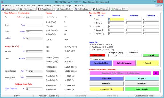
In Figure 42, the appropriate variables are ranged and the desired interval for the iteration has been entered.

Figure 42

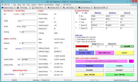
Figure 43 shows the table generated for the drag factor (adjusted for braking) solving for the Initial Speed keeping the Distance and Final Speed constant as selected in Figure 42.

Figure 43

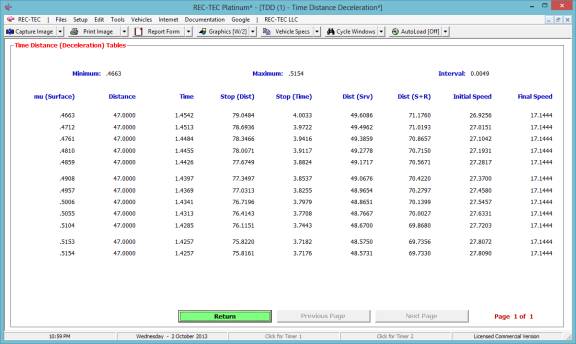
Figure 44

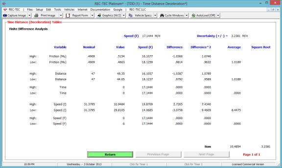
Figure 44 shows a finite difference analysis for the final speed (speed at contact with the pedestrian) based on ranging the Drag Factor, Distance and Initial Speed generating an uncertainty value of 6.064 M/H.

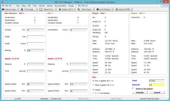
Module 4: Time - Distance – Multiple Vehicle

(Table of Contents)

Overview: This module computes comparative data for two vehicles in two individual acceleration, deceleration or constant velocity events and offers animation of the maneuver.

At the REC-TEC pull down menu, select Time - Distance > Multiple Vehicles and the Time Distance Multiple Vehicles screen appears (Figure 45).

Figure 45

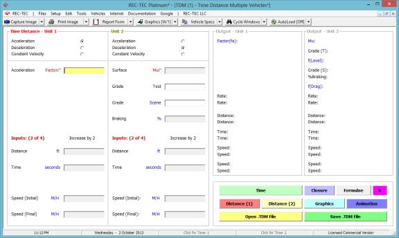
Required Inputs

The required input data depends on the user-selected maneuver for each vehicle or object. Single-Surface Acceleration and Single-Surface Deceleration modules can be referenced for information on the required input data for these maneuvers. Constant Velocity will require the Initial Speed and the Final Speed as inputs, and they must be identical.

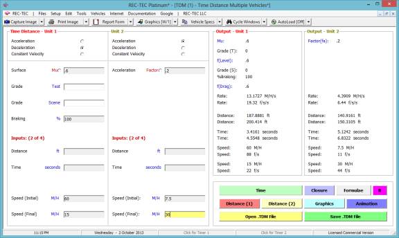
Example 1: Vehicle 1 decelerates from 60 miles per hour to a final speed of 15 miles per hour (striking vehicle 2). The Mu value is 0.6 and the grade is zero. The braking is 100%. Vehicle 2 accelerates from 7.5 miles per hour to a final speed of 30 miles per hour (striking vehicle 1). The acceleration factor is 0.2.

This module allows some unique options such as CLOSURE, which can help investigate the sight triangle between the two units involved. Either vehicle can be studied for any time or distance before the event in question, be it a collision, stop, or any point under consideration

For this problem, two vehicles will be taken into collision. Tables can be generated to study what happened before impact. With the ability to look at units in any combination of acceleration, deceleration, or constant velocity, any situation can be analyzed.

This section can be used to analyze vehicles, or vehicles and pedestrians in collision. This section can also be used to study the effects of different values for the same vehicle (side by side).

Figure 46

1. How fast was Vehicle #2 going when vehicle #1 was 1.5 seconds from impact?

2. How far from impact was Vehicle #1 when Vehicle #2 was 5 seconds from impact?

 Figure 47

If the vehicles end together at Time = 0, and a .5 second time interval is used, a speed table can be created that will answer the question.

The answer to question #1 is 23.4136 M/H (Figure 48)

Figure 48

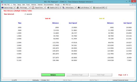
The answer to question #2 is 327.267 feet. (Figure 48)

3. When Vehicle #2 was 25 feet from impact, what was the speed of vehicle #1?

Figure 49

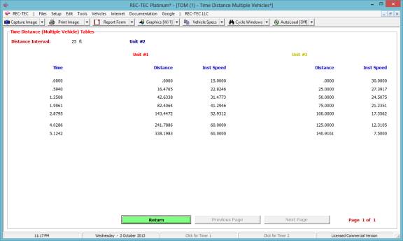
The answer to question #1 is 22.8246 M/H (Figure 49)

The Closure button computes data on the triangle using the two vehicles and impact.

Figure 50

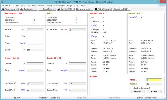
The Execute button displays (Figure 51) the triangular relationship defined by the angles entered in the blocks on Figure 50.

Figure 51

The Graphics button (Figure 46) brings up a menu (Figure 52) controlling the graphics curves (Time or Distance and the values involved) displayed on the screen (Figure 53).

Figure 52

Figure 53 shows the time curves for the greater time of the acceleration.

Figure 53 (Time)

Selecting Distance on the menu shown on Figure 54 and increasing the total distance from 187.8881 feet to 250 feet shows the graphics on Figure 55.

Figure 54

Figure 55 shows the distance curves for the increased distance of 250 feet.

Figure 55

The Animation button (Figure 46) brings up a menu (Figure 56) controlling the way animation is displayed on the screen.

Figure 56

After engaging the options of choice on this menu (Figure 56), the Execute button will initiate the animation (Figure 57).

Figure 57

Example 2: Vehicle 1 decelerates from 60 miles per hour to a final speed of zero. The drag factor is 0.72. Vehicle 2 decelerates from 60 miles per hour to a final speed of zero. The drag factor is .61. Vehicle 2 is "Trailing" 100 ft. behind Vehicle 1. Vehicle 2 has a 1.5 second perception reaction time (PRT) when Vehicle 1 brakes. There is no grade and the braking is 100% for both vehicles.

Figure 58 

Once the problem is setup up, select Animation. Select "From Start" and use the parallel format. Answer the remaining questions using the information listed above. Select compute for TIME.

Figure 59

Figure 60

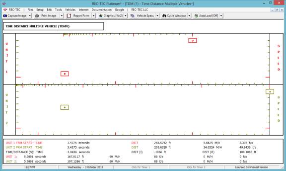
Do the vehicles hit? At what speed?

Vehicle 1______________________

Vehicle 2______________________

Example 2A: How would the answer change if the PRT was 2 seconds and the trailing distance was 75 feet?

Do the vehicles hit? At what speed?

Vehicle 1______________________

Vehicle 2______________________

Example 2B: How would the answer change if the PRT was 1 second and the trailing distance was 150 feet?

Do the vehicles hit? At what speed?

Vehicle 1______________________

Vehicle 2______________________

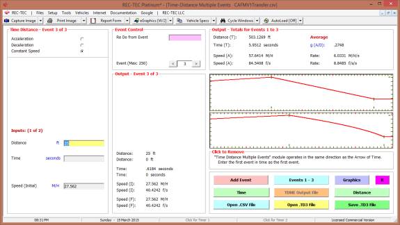
Module 5: Time - Distance – Multiple Events

(Table of Contents)

Overview: This module computes the intermediate and final speed, distance and time data for multiple (250) acceleration, deceleration, or constant velocity events. The module will also decode and assist in analyzing CDR data that may be presented in unfamiliar configurations such as metric accelerations (meters/second/second) in Toyota vehicles, or others similarly equipped by changing the primary input to meters/second and changing acceleration to rate instead of factor. After saving the file (as a precaution) changing the configuration or opening the file at a later date with a different configuration, will convert it to any configuration desired. Graphics, Tables, and Time and Distance breakdowns are available.

At the REC-TEC pull down menu, select Time - Distance > Multiple Events and the Time Distance Multiple Events screen appears (Figure 61).

Figure 61

Required Inputs

The required input data depends on the user-selected maneuver for each vehicle or object. Single-Surface Acceleration and Single-Surface Deceleration modules can be referenced for information on the required input data for these maneuvers. Constant Velocity will require the Initial Speed and either a Distance or a Time as inputs.

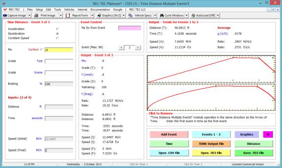
Figure 61 (Event Control) shows a Re Do from Event Entry Box. Enter event number that requires a change. If a correction is required, it will be necessary to go back to the event with the error and proceed from that point.

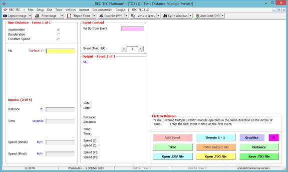
Example 1: A vehicle accelerates from a stop (fa = .2) for 25 feet. It then coasts (f = .01) for 15 feet before decelerating (f = .6) to a final speed of 5 miles per hour.

Note: As shown in Figure 61, the Time - Distance Multiple Events module operates in the same direction as the Arrow of Time. Enter the first event in time as the first event.

Figure 62

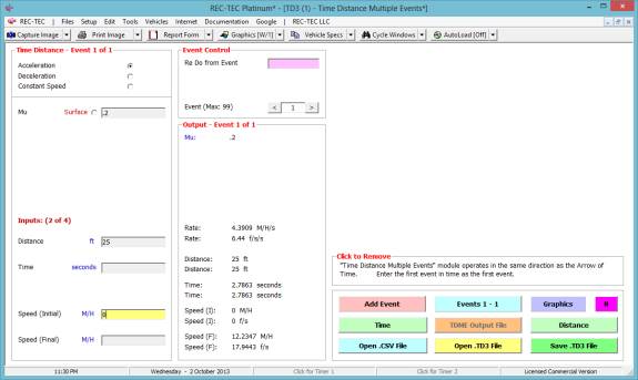
Figure 62 shows the entry data for the first of three events.

Figure 63

Click Add Event to proceed to next event. Figure 63 shows the data entry for the second of the three events. Output totals for the first two events appear in the upper right of the screen.

Figure 64

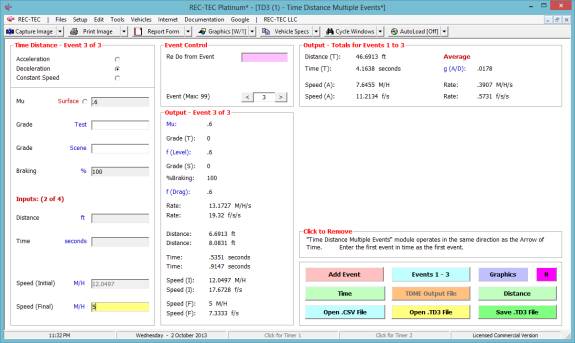
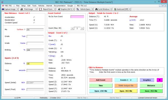
Click Add Event to proceed to next event. Figure 64 shows the data entry for the third of the three events. Output totals for the first three events appear in the upper right of the screen.

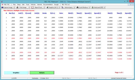
Figure 65

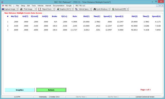
Figure 65 shows the table created using the Events (1-3) button.

Figure 66 shows a table created by using a time interval of 0.5 seconds.

Figure 66

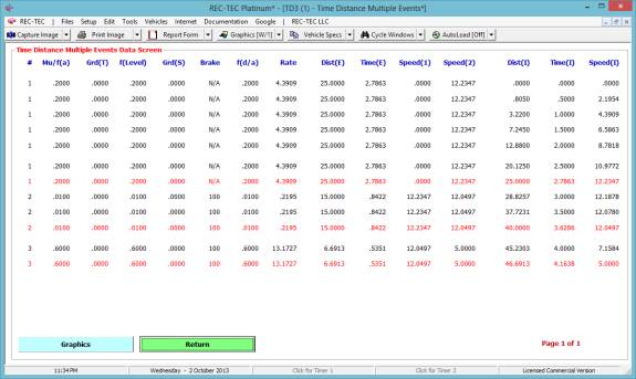
Figure 67 shows a table created by using a distance interval of 5 feet.

Figure 67

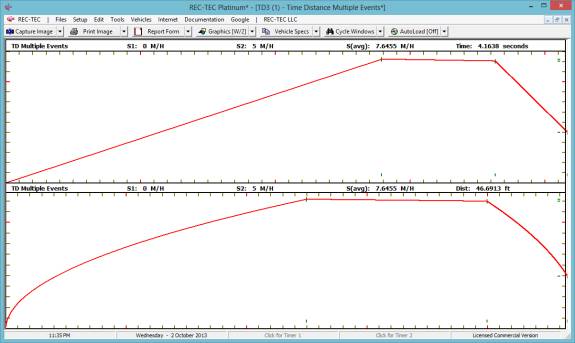
If Graphics is selected from the input screen, the graphics appear with the data incorporated into the same screen (Figure 68). If the [Esc]ape key is pressed with the graphics on the data screen, the Graphics will go to full screen as shown in Figure 69.

Figure 68

Use the [Esc]ape key to display the Graphics curves in full screen mode.

Figure 69

Event Control will dictate the data displayed in the Events, Time, Distance, and Graphics buttons, as the Event number can be set controlling what is displayed.

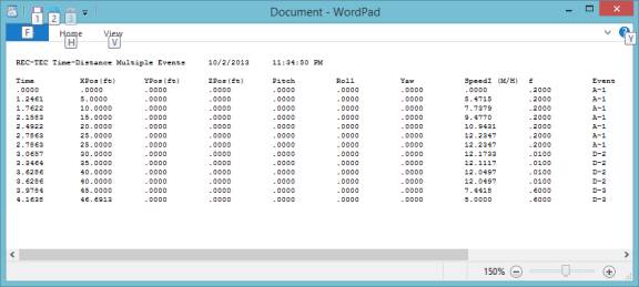
The TDME button will create an output file matching the last table run in either Time or Distance.

Figure 70

What is the total time for this example? What is the total distance for this example?

Example 2: A vehicle goes through the following maneuvers:

1. Acceleration factor = .2 Initial speed = 30 M/H Final speed = 60 M/H

2. Constant speed Distance = 264 ft

3. Acceleration factor = .2 Initial speed = 60 M/H Final Speed = 75 M/H

4. Constant speed Distance = 300 ft

5. Deceleration factor = .3 Initial speed = 75 M/H Final Speed = 60 M/H

6. Deceleration factor = .6 Initial speed = 60 M/H Final Speed = 45 M/H

7. Constant speed Time = 5 seconds

8. Deceleration factor = .6 Initial speed = 45 M/H Final Speed = 0 M/H

9. Stopped for 30 seconds

10. Acceleration factor = .2 Initial speed = 0 M/H Final Speed = 45 M/H

11. Constant speed Time = 5 seconds

12. Acceleration factor = .3 Initial speed = 45 M/H Final Speed = 60 M/H

13. Constant speed Distance = 400 ft

14. Deceleration factor = .75 Initial speed = 60 M/H Final Speed = 0 M/H

Note: All braking is at 100%.

Figure 71

What is the total distance?

What is the total time?

What is the Average Speed for the sequence?

What is the total distance at the end of Event 12?

What is the total time at the end of Event 12?

What is the Average Speed for the sequence at the end of Event 12?

Figure 72

The Time and Distance curves for all 14 events are shown in Figure 73.

Figure 73

Module 6: Time - Distance – Multiple Surfaces

(Table of Contents)

Overview: This module computes the intermediate speed, final speed, distance and time data over multiple surfaces in an acceleration, deceleration or at constant velocity.

At the REC-TEC pull down menu, select Time - Distance > Multiple Surfaces and the Time Distance Multiple Surfaces screen appears (Figure 74).

Figure 74

Required Inputs

The required input data depends on the user-selected maneuver for each vehicle or object. Single-Surface Acceleration and Single-Surface Deceleration modules can be referenced for information on the required input data for these maneuvers. Constant Velocity will require the Initial Speed and either a Distance or a Time as inputs.

Example 1: A vehicle decelerates from an unknown speed (f = .72) for 25 feet. It then decelerates over a second surface (f = .6) for 15 feet before decelerating 30 feet (f = .3) to a stop. All Braking is 100%. What is the time and distance?

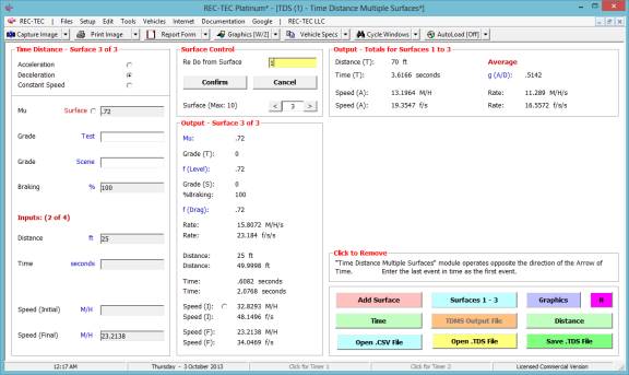
Note: As shown in Figure 74, the Time - Distance Multiple Surfaces module operates opposite the direction of the Arrow of Time. Enter the last event in time as the first event.

In Figure 75, the last event (deceleration to a stop) is entered as the first event. Click Graphics to show them as seen in Figure 75.

Figure 75

Click Add Surface to proceed to next event. In Figure 76, the next event (event #2) is entered as the second event.

Figure 76

Click Add Surface to proceed to next event. In Figure 77, the first event (initial deceleration) is entered as the last event.

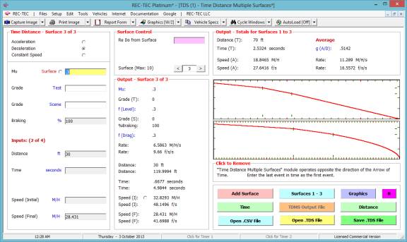
Figure 77

Note the “Radio Button” Next to the Initial Speed (Primary) – See Page 11 for details.

Press [Esc]ape to show (or clear) the full screen graphics of all three events as displayed in Figure 78.

Figure 78

Press Surfaces 1-3 to show the data for all three events (Figure 79).

Figure 79

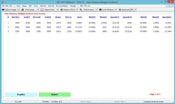
Figure 80 is the Time interval (0.5 seconds) breakdown of all three maneuvers. This table also shows the associated data at the change of events.

Figure 80

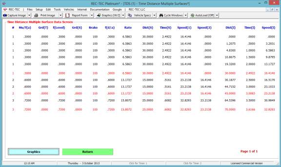
Figure 81 is the Distance interval (10 feet) breakdown of all three maneuvers. This table also shows the associated data at the change of events.

Figure 81

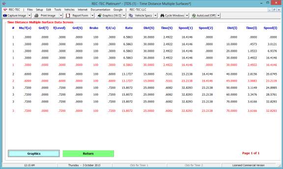
Press TDMS Output File to create the file (TDMSO.out) as shown in Figure 82.

Figure 82

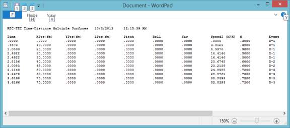
Figure 83 (Surface Control) shows a Re Do from Surface #1. If a correction is required, it will be necessary to go back to the event with the error and proceed from that point.

Figure 84 shows the effects of entering the events in reverse order. While the initial speed and total distance are the same, the times, including the total time are not.

Figure 83

Please compare the data in Figure 77 with the data (and graphics) in Figure 84.

Figure 84

Module 7: Time - Distance – Time - Distance (Acc~Dec)

(Table of Contents)

Overview: This module computes detailed information on the Speed, Distance and Time of an Acceleration-Transition-Deceleration event.

At the REC-TEC pull down menu, select Time - Distance > Time - Distance (Acc~Dec) and the Time - Distance (Acc~Dec) screen appears (Figure 85).

Figure 85

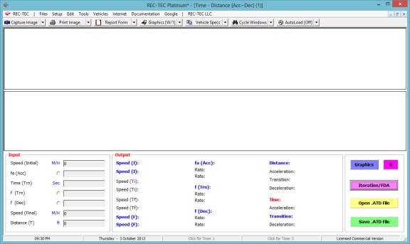
Required Inputs

· Speed (Initial) – Speed at start of maneuver

· fa (Acc) – Acceleration factor (Zero if no acceleration)

· Time (trn) – Transition time

· f (Trn) – Deceleration factor during Transition (rolling resistance?)

· f (Dec) – Deceleration factor (Zero if no acceleration)

· Speed (Final) – Speed at end of maneuver

· Distance (T) – Total Distance of maneuver

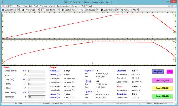
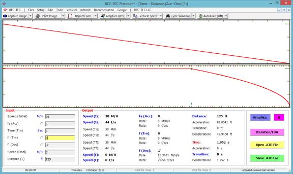
Example 1:

• Initial Speed = 0
• f(acc) = .2
• Time = 1.5
• f(trn) = .01
• f(dec) = .7
• Final Speed = 5 M/H
• Distance = 125

Figure 86

The Iteration/FDA button brings up the following menu.

Figure 87

Figure 88

The data in Figure 88 will automatically be saved as “Lastfile.ATD” when the program is exited. This data may automatically be loaded if the AutoLoad is On. It may be manually reloaded using the Open.ATD button. Using this option, the top bar of the program screen will show the name of the loaded file (Figure 89).

Figure 89

Figure 90 displays the Iteration table for the parameters shown in Figure 88.

Figure 90

Figure 91 displays the Finite Difference Analysis for the parameters shown in Figure 88.

Figure 91

Example 2:

• Initial Speed = 30
• f(acc) = 0
• Time = 0
• f(trn) = 0
• f(dec) = .7
• Final Speed = 0
• Distance = 125

As shown in this example, this module does not require much in the way of information to generate a solution. This module was primarily designed to assist in the analysis of intersectional collisions involving vehicles and pedestrians. It can be adapted to various situations.

Figure 92

Module 8: Time - Distance – Time - Distance – Omni

(Table of Contents)

Overview: This module computes Acceleration/Deceleration factors and rates, Time, Distance, and/or Speed as appropriate based on supplied information. It will create a table of user-developed research data (pedestrian/vehicle study) for speed, time, distance and/or acceleration/deceleration rates, which automatically integrates into the Statistical Range (Monte Carlo) module in REC-TEC allowing additional analysis (mean, range, variance, upper and lower bounds).

This very powerful module does all of the basic computations of the Acceleration/Deceleration Factor, Acceleration Single Surface and Deceleration Single Surface modules of the program in a single module. It now provides for Graphics, Iteration and Finite Difference Analysis. It does not allow for Lateral Distance (Swerve / Lane Change) computations, Grade, or Braking adjustments.

At the REC-TEC pull down menu, select Time - Distance > Time - Distance – Omni and the Time - Distance – Omni screen appears (Figure 93).

Figure 93

Required Inputs

The “required” input data depends on the user-selected maneuver. An Acceleration/Deceleration factor is not required. Single-Surface Acceleration and Single-Surface Deceleration modules can be referenced for information on the required input data for these maneuvers. Constant Velocity will require the Initial Speed and either a Distance or a Time as inputs.

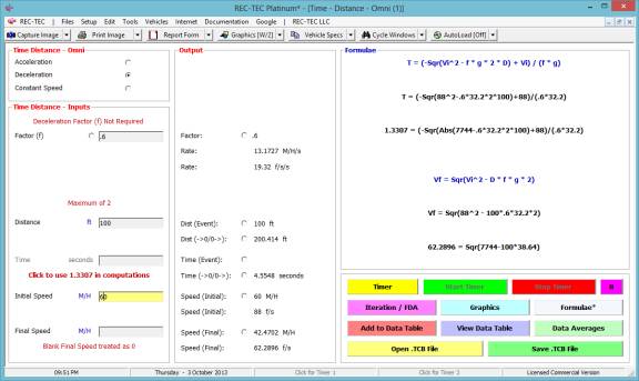
Example 1: A vehicle decelerates for 100 feet to a final speed of zero (0).

1. What is the initial speed and time if the deceleration factor is .65?

2. What is the deceleration factor and initial speed if the time is 3 seconds?

3. What is the deceleration factor and time if the initial speed is 45 M/H?

Time - Distance – Omni easily answers all three questions in the same module.

Figure 94

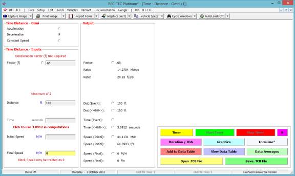
The answer to question #1 is 44.1131 M/H and 3.0912 seconds (Figure 94).

Figure 95

The answer to question #2 is 0.6901 (f) and the initial speed is 45.4545 M/H (Figure 95).

Figure 96

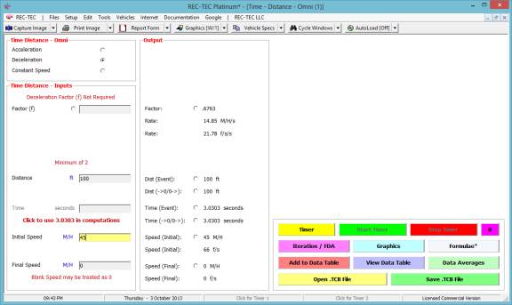
The answer to question #3 is 0.6763 (f) and the time is 3.0303 seconds (Figure 96).

Time - Distance – Omni also handles accelerations.

Example 2: A vehicle accelerates for 100 feet from an initial speed of zero (0).

4. What is the final speed and time if the acceleration factor is .2?

5. What is the acceleration factor and initial speed if the time is 5.5 seconds?

6. What is the acceleration factor and time if the final speed is 25 M/H?

Time - Distance – Omni easily answers all three questions in the same module.

Figure 97

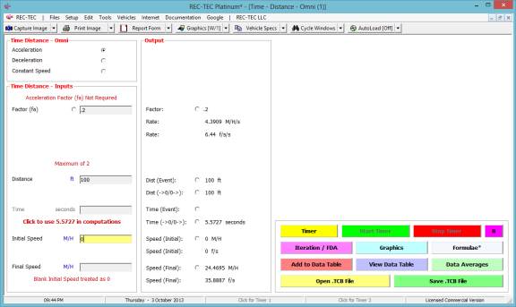
The answer to question #1 is 24.4695 M/H and 5.5727 seconds (Figure 97).

Figure 98

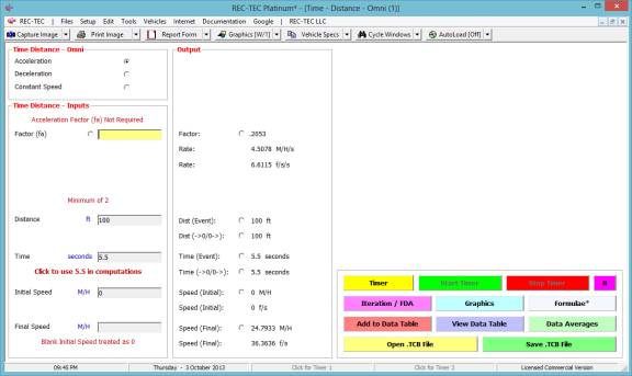
The answer to question #2 is 0.2053 (fa) and the initial speed is 24.7933 M/H (Figure 98).

Figure 99

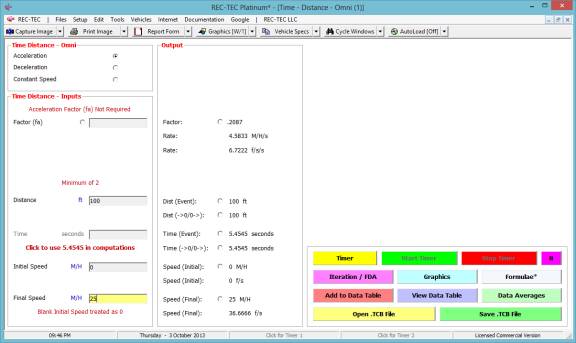
The answer to question #3 is 0.2087 (f) and the time is 5.4545 seconds (Figure 99).

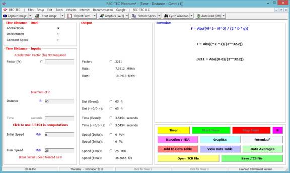
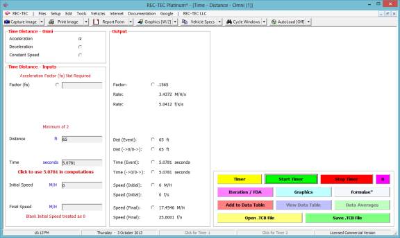
Change the Distance to 65 and show the Formula.

Figure 99B

Select Iteration by Factor and range from .2211 to .4211 by .05.

Figure 99C

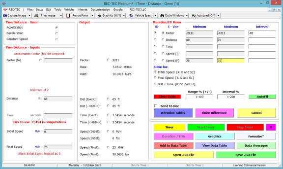
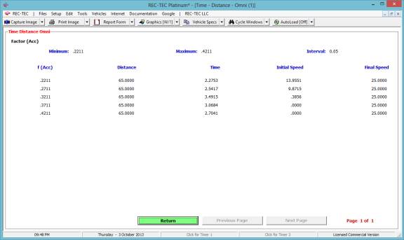
Results are shown in Figure 99D

Figure 99D

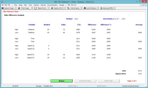
Using the setup in Figure 99C, do a Finite Difference Analysis for Factor.

Figure 99E

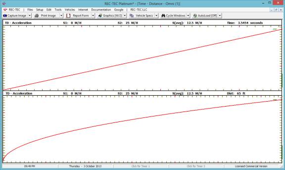
Show the Graphics curves for the Problem shown in Figure 99.

Figure 99F

Decelerate from 60 M/H for 100’ using a deceleration factor of .6 showing the Formulae and Results.

Figure 99G

Time - Distance – Omni can also be used to time vehicles over a known distance to calculate speeds. This works with vehicles accelerating from a traffic control device, tollbooth, or a truck weight station. It can be used to time pedestrians crossing streets or other scenarios.

Example 3: Create a table of vehicles accelerating from a stop sign and clearing a point outside of the intersection (65 feet).

Note: The following screen captures have not been updated as the modifications shown above do not change these screens.

· Timer button – Initiates the Timer mode but does not start the Timer.

· Start Timer button – Starts the Timer (Enter will also start the Timer in Timer mode).

· Stop Timer button – Stops the Timer (Enter will also stop the Timer in Timer mode).

· Add to Data Table button – Transfers the data from the current “run” to the Data Table.

· Data Table Averages – Displays the averages of the Entries in the Data Table.

· View Data Table – Shows Data Table and allows selection of entries for further processing in the Statistical Range (Monte Carlo) module.

In the following example, 10 timing runs are simulated and entered into the data table.

In this Acceleration Example a vehicle is timed over 65 feet from a stop. Click on Timer. Click on Start Timer (or use Enter) to Start the Timer. Click on Stop Timer (or use Enter again) to Stop the Timer and display the results for this run.

If the Run was good, then Click Add to Data Table. If for some reason the Run went bad, simply ignore it and Time the next Vehicle.

The data table is averaged as the numbers are entered. After the runs are completed, the data table is displayed. The Speed (M/H) is selected for further analysis and written as a file, which is then opened in the Statistical Range (Monte Carlo) module.

The first run is displayed in Figure 100.

Figure 100

The first run has been transferred into the data table and the Data Table Averages are shown in the upper right frame.

Figure 101

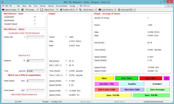
Figure 102 shows the averages for all 10 runs.

Figure 102

Figure 103 displays the Data Table with all of the arrays. The Speed2 (M/H) column is tagged for transfer into the Statistical Range (Monte Carlo) module for further analysis.

Figure 103

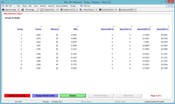
Figure 104 displays the Statistical Range (Monte Carlo) screen showing the graphics for a 100,000-point Monte Carlo analysis for Final Speed.

Figure 104

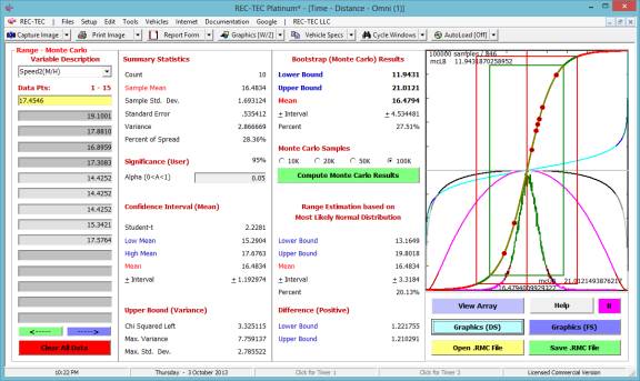
Figure 105 shows the graphical display of the various curves in the Statistical Range (Monte Carlo) module. The circles are the points from the data table that were transferred in order to make the analysis.

Figure 105

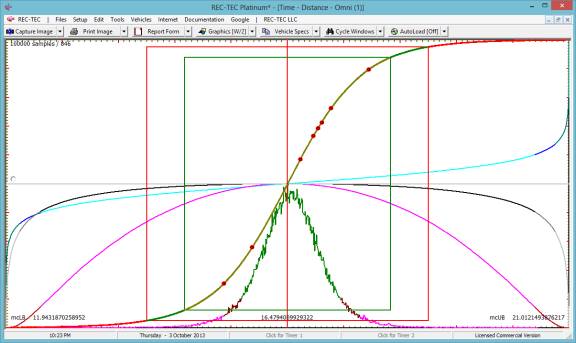
Figure 106 is the comma-delimited file that was created from the Data Table (Figure 103).

Figure 106

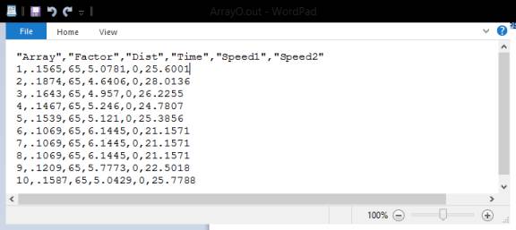
Figure 107

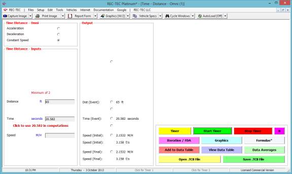
Figure 107 is an example of how Time - Distance – Omni can be used to time pedestrians (or any moving object) to compute the average speed involved. This data can be transferred into an endless array data table for further analysis in the Statistical Range (Monte Carlo) module.

The Time - Distance – Omni is a real workhorse in analyzing many time-distance problems. It has the versatility and power to become one of your most popular tools.

Module 9: Collision Avoidance – Braking Maneuvers

(Table of Contents)

Overview: This module computes speed, time and distance required to either stop before striking target vehicle, or decelerate enough to allow crossing target vehicle to escape.

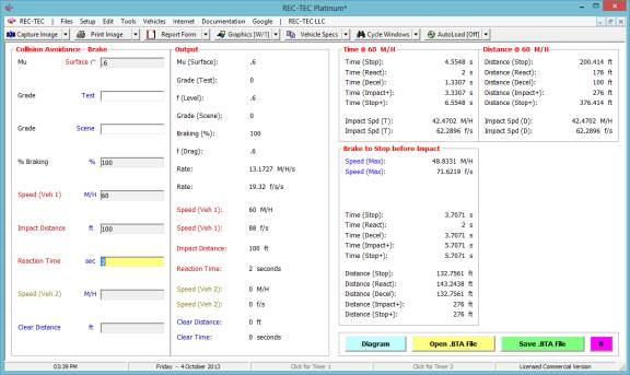
At the REC-TEC pull down menu, select Collision Avoidance > Braking Maneuvers and the Collision Avoidance – Braking Maneuvers screen appears (Figure 108).

Figure 108

Required Inputs

· Mu (Deceleration) - required

· Grade (Test) – not required (default is zero)

· Grade (Scene) – not required (default is zero)

· Braking (%) – required

· Speed (Veh 1) – Initial Speed of Vehicle 1

· Impact Distance – Distance from End of Reaction Time to Point of Impact

· Reaction Time – Actual or Imputed

· Speed (Veh 2) – Speed of Vehicle 2

· Clear Distance – Distance Vehicle 2 must travel to avoid contact

Example 1: A vehicle decelerates from 60 M/H on a surface with a .6 coefficient of friction. There is no grade and the vehicle braking is 100 percent. After a Perception-Reaction time of two seconds, it travels 100 feet striking vehicle #2. Vehicle #2 is traveling at 30 M/H. If vehicle #2 had traveled 10 more feet, it would have cleared the path of Vehicle #1.

1. What is the maximum speed of Vehicle 1 for it to stop before contacting Vehicle #2?

2. What is the maximum speed of Vehicle 1 for it to pass safely behind Vehicle #2?

3. What is the speed of Vehicle 1 as it passes behind Vehicle #2 in question #2?

Figure 109

Figure 110

As can be seen in Figure 109, the only option offered by this module is showing the Diagram (Figure 110). The data generated by this module is a bit overwhelming at first glance.

The F1 (Help) file will help decipher the output data (Figure 109) and placing the cursor on a particular piece of data will display a “ToolTip” describing the data.

While there is a huge amount of information on Figure 108, the diagram (Figure 109) helps to filter the data making the problem easier to understand. Unfortunately, a closer look at Figure 110 may raise more questions than it answers. For example, the entered distance between the PRT and impact is 100 feet (Figure 108), yet in Figure 109 the distance is shown as 132.7561 feet for the STOP scenario and 107.6771 feet for the CLEAR scenario.

In the data entry, the distance is 100 feet. This 100-foot distance is the deceleration distance from an initial speed of 60 M/H, resulting in a collision. Given the same total distance for the reaction time and the deceleration, the module computes that if the initial speed was 48.8331 M/H, then Vehicle #1 could come to a complete stop just short of striking Vehicle #2. Using this same distance and an initial speed of 57.3827 M/H, Vehicle 1 could have decelerated and passed safely behind Vehicle #2 without a collision.

Understanding the principles put forth in the above paragraph, the data shown on Figure 109 should make more sense. All three maneuvers, the collision, the stop and the clear must all use the same total distance. The times will vary with the different speeds, but the total distance available is the same in all three.

The data entered into the problem must describe a collision. If the distance entered is over 200.414 feet, there never would be a collision as Vehicle 1 would be able to stop before striking Vehicle 2 and there would be no reason to use this or any other module in the program. Once that collision is described, the module will compute the maximum possible speeds both to STOP, and to CLEAR.

Included in the data shown on Figure 109 is the impact speed based on both time and distance for the input speed of 60 M/H. The result is a collision speed of 43.4702 M/H. In the Brake to Clear frame on Figure 108, the Speed (Clear) data is the speed that Vehicle 1 would have at the time it passed behind Vehicle 2.

Example 2: In this example, use the same data for Vehicle 1. For Vehicle 2 change the speed and the clear distance both to zero (0).

Figure 111

With these changes in place, there can be no solution for questions 2 and 3. The diagram (Figure 112) shows the impossibility of the solution.

Figure 112

Module 10: Collision Avoidance – Collision Analysis

(Table of Contents)

Overview: This module computes the speeds, times and distances during which the vehicles are exposed contact and during which contact will actually occur.

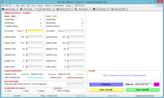
At the REC-TEC pull down menu, select Collision Avoidance > Collision Analysis and the Collision Avoidance – Collision Analysis screen appears (Figure 113).

Figure 113

Data Entry: Entries for either Vehicle can consist of Acceleration, Deceleration or Constant Speed and will contain two or more of the following data entry blocks within the two leftmost frames:

· ‘g’ Acc/Dec (Acceleration/Deceleration – required)

· Speed (Initial)

· Speed (Final)

· Reaction Time

· Distance – Distance from front of vehicle to center of vehicle paths at impact

· Length (LOV)

· Width (WOV)

· Intercept Angle – Angle between vehicles

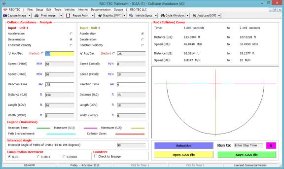
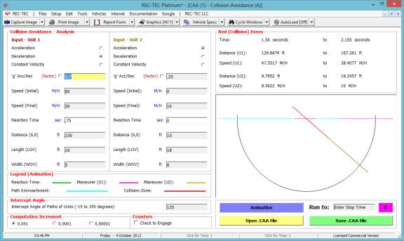
Example 1: At time zero, Vehicle 1 starts 150 feet from point (0,0). After a 0.75 second reaction time, it begins decelerating at 0.7 g from an initial speed of 60 M/H to a final speed of 30 M/H. Vehicle 1 is 16 feet long and 5 feet wide. Vehicle 2 starts 15 feet from point (0,0). At time zero, it begins to immediately accelerate at 0.25 g from a stop to a final speed of 10 M/H. Vehicle 2 is 18 feet long and 6 feet wide. The intercept angle of the paths of the units is 90 degrees. The paths will cross at point (0,0)

What is the start time and end time during which the vehicles are trying to occupy the same space?

What is the start distance and end distance during which the vehicles are trying to occupy the same space?

What is the start speed and end speed during which the vehicles are trying to occupy the same space?

Figure 114

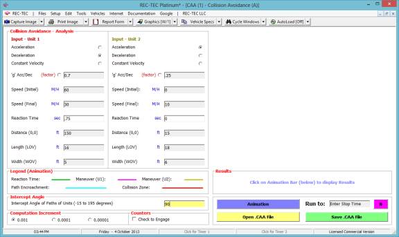
Figure 115

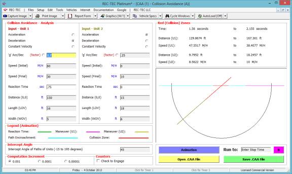
Example 2: With a 45 degree intercept angle, how would the answers differ from those in Example 1.

Figure 116

Example 3: With a 135 degree intercept angle, run the problem with a stop time of 1.56 seconds and show the results.

Figure 117

Module 11: Collision Avoidance – Following Maneuvers

(Table of Contents)

Overview: This module computes the speed, time and distance at which a maximum rate deceleration or an evasive maneuver must begin in order to match the speed of the (accelerating, decelerating or constant-velocity) lead vehicle, thus preventing a collision.

At the REC-TEC pull down menu, select Collision Avoidance > Following Maneuvers and the Collision Avoidance – Following Maneuvers screen appears (Figure 118).

Figure 118

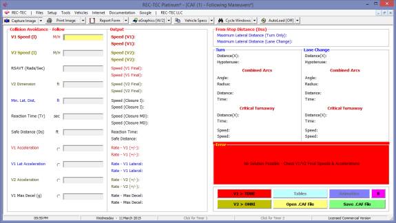
Required Inputs:

· V1 Speed (I) – Following (Bullet) Vehicle at Start of Maneuver

· V2 Speed (I) – Leading (Target) Vehicle at Start of Maneuver

· RSAVT (Rads/Sec) – Relative Subtended Angular Velocity Threshold in Radians per Second

· V2 Dimension – Height or Width Cue for Subtended Angular Rate Change Computation (Height/Width of Trailer or Distance between tail lights

· Min Lat. Dist. – Minimum Lateral Distance (Turn / Lane Change)

· Reaction Time – Time before V1 reacts to V2 maneuvers

· Safe Distance – Separation Distance Between Vehicles at Speed match

· Acceleration (+/-) (V1) – Acceleration Factor if V1 Accelerating (+/-) prior to entering Max rate Deceleration

· Lateral Accel. (V1) – Lateral (Y-Axis) Acceleration Factor - Required

· Acceleration (V2) – Acceleration Factor (X-Axis) if V2 Accelerating (+/-)

· Maximum Decel. (g) – Maximum Available Deceleration (g)

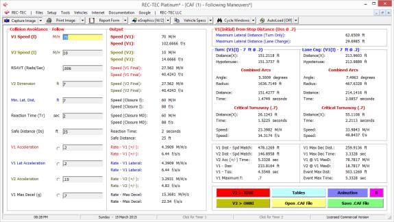
Example 1: Vehicle 1 (bullet) is traveling at 70 M/H. Vehicle 2 (target) is traveling in the same direction at 10 M/H. V2 width is 7 feet (used with RSAVT). The minimum lateral distance to avoid collision is also 7 feet. Vehicle 1 is capable of accelerating laterally at 0.2 g. Vehicle 2 is accelerating at 0.15 g. The maximum deceleration factor for Vehicle 1 is 0.7g. Reaction time for Vehicle 1 is 2 seconds and distance required between vehicles at speed match is 25 feet. RSAVT is 0.006.

On Figure 119 there are computations that would be difficult to solve for without this module as you are effectively trying to land a satellite on a comet that could be accelerating (positive/negative).

Figure 119

Primary Output:

1 V1 Dist – Contact (Spd Match): V1 - Distance to Contact (Spd Match) from Time Zero (0)

2 V2 Dist – Contact (Spd Match): V2 - Distance to Contact (Spd Match) from Time Zero (0)

3 V2 Acc (+/-) Time: Includes time V2 is Accelerating (+/-) before V1 begins Decelerating

4 V1 – Dss: Distance to Decelerate from Initial Speed at Maximum f

5 V1 – Tss: Time to Decelerate from Initial Speed at Maximum f

6 V1 Maximum f: Maximum Deceleration Factor (g)

7 V1 Max Dec Dist.: Distance Required to match V2 Speed - Maximum Deceleration (g)

8 V1 Max Dec Time: Time Required to match V2 Speed - Maximum Deceleration (g)

9 V1 @ V1 MaxD: V1 Speed (Primary) at V1 Maximum Deceleration Start

10 V2 @ V1 MaxD: V2 Speed (Primary) at V1 Maximum Deceleration Start

11 Event Max Dist.: Maximum Distance from Time Zero (0)

12 Event Max Time: Maximum Time from Time Zero (0)

Animation – The display (Figure 115) shows the acceleration curves for both vehicles in the upper block and the Turn (upper middle block) and Lane Change (lower middle block). Time (top scale) and Distance (bottom scale) is shown for all three curves. Animation may be stopped and resumed using the mouse or the spacebar. [Esc] to Exit

Tables – Tables show either, the f required to clear (Match V2 Speed) and Closing Speed at Maximum Available Deceleration from Time frame, or the Subtended Angle (Radians) and Rate of Change of the Subtended Angel in Radians/second. Both tables display Time in user selectable increment to Point of Contact. Table data includes instantaneous speeds for V1, V2, Closing Speed, required distance for Turn and Lane Change, Separation Distance between Vehicles and Time to Impact and Distance traveled by V1 and V2.

Figure 120

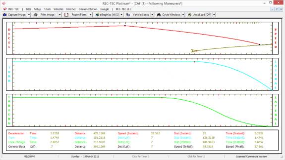
Figure 121

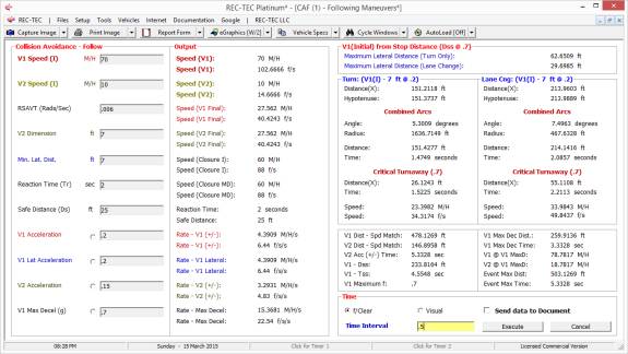
Figure 121 includes the menu choice (f/Clear or Visual) and the time interval for the Table. Figure 122 displays the f/Clear table and Figure 123 displays the Visual (RSAVT) table.

Figure 122

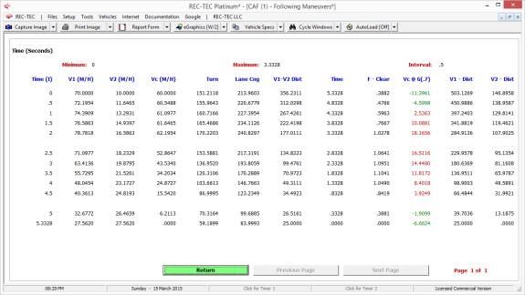
Figure 123

On both tables (Figures 122 fClear and 123 Visual), the value in the 10^th column changes color from green to red. On Figure 122, the column labeled Vc@f(.7) shows the collision speed at the maximum deceleration rate. A negative speed value would mean that the vehicle (V1) could be backing up at that speed if the deceleration (acceleration) values were maintained.

Figure 123A

Figures 123A and 123B show V1 data automatically transferred to Time Distance Multiple Events for further analysis and as a cross check on both the math and the graphics.

Figure 123B

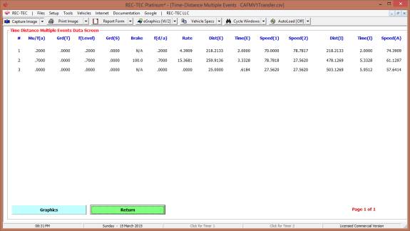
Figure 123C

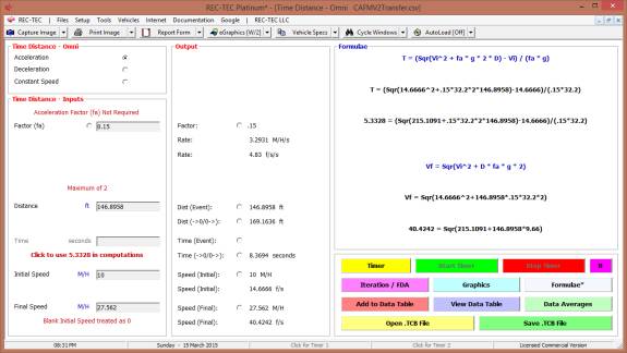
Figure 123C shows V2 data automatically transferred to Time Distance Omni for further analysis and as a cross check on the math with graphics diagrams available.

Module 12: Collision Avoidance – Passing Maneuvers

(Table of Contents)

Overview: This module computes the Time and Distance required to complete a passing maneuver.

Note: REC-TEC uses a Circle as the model in computing Turn information. All of the other popular Turn formulae use a Parabola as their model. The result is that the term “lateral” has two very different connotations in discussing turning accelerations. In REC-TEC (Circular) the “lateral” acceleration is always perpendicular to the instantaneous direction of the vehicle except in this module where the user is given a choice. In the other formulae (Parabolic) the term “lateral” references the initial direction of travel of the vehicle and the acceleration is always perpendicular to that initial direction.

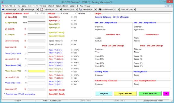
At the REC-TEC pull down menu, select Collision Avoidance > Passing Maneuvers and the Collision Avoidance – Passing Maneuvers screen appears (Figure 124).

Figure 124

Required Inputs:

· Pass ( ) L ( ) R – V1 past to Left or Right of V2 (used for Diagram and Animation output files)

· Circle ( ) Parabola ( ) – Selects Circular or Parabolic formulae for lane changes (Turns)

· V1 Speed (I) – Speed at start of Maneuver

· V2 Speed (I) – Speed at start of Maneuver

· V1 Length

· V2 Length

· Lane Centers (D) – Distance between Lane centers

· Separation (I) – Initial Separation Distance (X-Axis) between Vehicles after first Lateral acceleration (lane change)

· Accel (V1) – Initial – Initial Acceleration factor (X-Axis) if V1 accelerating

· Lat. Accel (V1-1) – Lateral (Y-Axis) Acceleration factor (required)

· Pass Accel (V1) – Passing Phase Acceleration factor (X-Axis) Required if V1 accelerating

· Pass Accel (V2) – Passing Phase Acceleration factor (X-Axis) Required if V2 accelerating

· Lat. Accel (V1-2) – Return Lateral (Y-Axis) Acceleration factor (required)

· Accel (v1) – Final – Final Acceleration factor (X-Axis) if V1 accelerating

· Separation (F) – Final Separation Distance (X-Axis) between Vehicles before second Lateral acceleration (lane change)

The Pass is broken down into three separate phases. Phase 1 is the initial longitudinal acceleration phase and the first lateral acceleration phase. Phase 2 is the passing phase. Phase 3 is the final longitudinal acceleration phase and the second lateral acceleration phase. (See Figure 126)

Example 1: Vehicle 1 is 16 feet long and Vehicle 2 is 17 feet long. Vehicle 2 is traveling at 50 M/H. Vehicle 1 is accelerating from 55 M/H at 0.05 g longitudinally while accelerating laterally at 0.1 g in order to pass Vehicle 2, which is 40 feet ahead. In the passing phase, Vehicle 1 will accelerate at 0.05 g and Vehicle 2 will accelerate at 0.025 g until Vehicle 1 is 60 feet in front of Vehicle 2 before accelerating laterally at 0.1 g while decelerating longitudinally at 0.01 g.

Figure 125

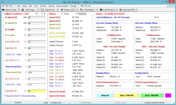
Figure 126

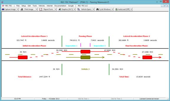
Total Distance is 1447.3757 feet. Total Time is 15.6639 seconds. Vehicle 1 final Speed is 67.1088 M/H.

Example 2: Remove the acceleration for Vehicle 2 in Example 2 and compare the Distance, Time, and final Speed from Example 1. (Figures below show “R” for Pass and “Circle” for formulae selection)

Figure 127

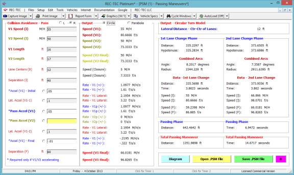
Figure 128

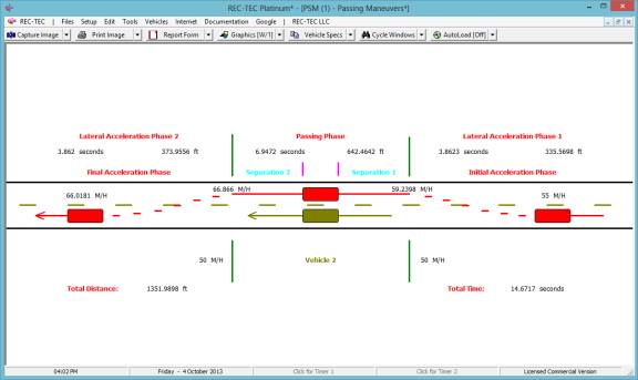
Total Distance is 1351.9898 ft, Total Time is 14.6717 seconds, and Vehicle 1 final Speed is 66.0181 M/H using “Circular” formulae.

Figure 128B

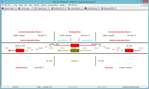
If using “Parabolic” formulae the Total Distance is 1342.7492 ft. Total Time is 14.6697 seconds. Vehicle 1 final Speed is 66.0174 M/H.

Module 13: Collision Avoidance – Turning Maneuvers

(Table of Contents) (Table of Contents)

Overview: This module computes data on Turn and Lane Change maneuvers, including braking during the turn, and compares different common formulae used in accident reconstruction.

At the REC-TEC pull down menu, select Collision Avoidance > Turning Maneuvers and the Collision Avoidance – Turning Maneuvers screen appears (Figure 129).

Figure 129

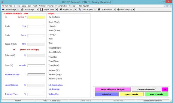
Required Inputs:

· Mu (Deceleration): – required

· Grade (Test): – not required (default is zero)

· Grade (Scene): – not required (default is zero)

· Speed (Initial): – Speed of vehicle - Computes Distances for Turn and Lane Change Maneuvers or (Enter zero to change)

· Distance (X): – Distance of Swerve (X-Axis) - Computes Initial Speed for Maneuver and Lane Change Distance data

· Time (Tr): – Reaction Time

· Acceleration (Lat): – Lateral Acceleration factor

· Lateral Distance: – Distance CG must move in Lateral Direction.

· Braking in Turn: – Optional – Percent of braking in Turn (must be less than 100)

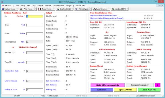
Example 1: A vehicle enters a turn at 60 M/H. It will accelerate laterally at 0.2 g. The Lateral distance is 12 feet. The road has a Mu (drag factor) of 0.7.

What is the distance traveled by the vehicle for the turn?

What is the time for this event?

What is the distance traveled by the vehicle for the lane change?

What is the time for this event?

What is the distance and time required for the vehicle to come to a full stop at a 0.7 g deceleration?

Figure 130

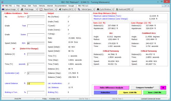
Turn: Time = 1.932 seconds | Distance Traveled = 170.0228 feet | Distance on X-axis = 169.4568 feet

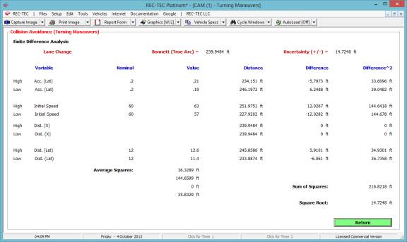
Lane Cng: Time = 2.732 seconds | Distance Traveled = 240.4237 feet | Distance on X-axis = 239.9484 feet

Full Stop: Time = 3.9041 | Distance Traveled = 171.7834 feet

Figure 131

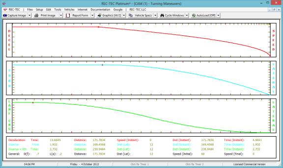
Figure 132 shows a comparison of the popular formulae used in accident reconstruction. Notes explain the differences in the focus of the formulae and the parameters inherent in their output.

Figure 132

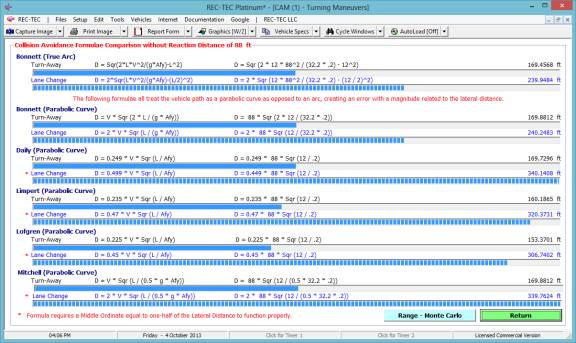
Figure 133

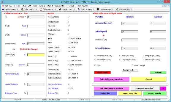
Figure 133 displays the Finite Difference Analysis Menu. The menu allows selection of any of the formulae used in the Formulae Comparison Chart. It also allows for the selection of a Turn or a Lane Change as the subject of the analysis. The results of a Turn are shown in Figure 134 and a Lane Change in Figure 135.

Figure 134

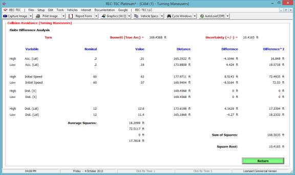
Figure 135

Example 2: This example will use the same basic information, but will add 20% braking during the maneuver.

What is the distance traveled by the vehicle for the turn?

What is the time for this event?

What is the distance traveled by the vehicle for the lane change?

What is the time for this event?

Figure 136

Turn: Time = 1.932 seconds | Distance Traveled = 161.6088 feet | Final Speed = 54.0614 M/H

Lane Cng: Time = 2.732 seconds | Distance Traveled = 233.5991 feet | Final Speed = 51.6025 M/H

Note: Braking in Turn – This option opens up two additional frames in the solution panel. The formulae for this solution are not used in Formulae Comparison, Animation, or in the Finite Difference Analysis.

Example 3: The times with and without braking in the turn and in the lane change are the same.

1. Prove that the time for the Turn and Lane Change is correct if the Distance computed is correct.

2. Explain why we know this is correct.

Answers

1A. 161.6088 / ((88 + 79.2901) / 2) = 1.932

1B. 223.5991 / ((88 + 75.6837) / 2) = 2.732

2. See Figures 136 and 137 – after you have tried to figure out the solution.

Figure 137

Allowing for a small difference between acceleration perpendicular to the initial direction of travel and acceleration perpendicular to the instantaneous direction of travel (REC-TEC), this is the same as the answer in 1A.

Figure 138

Allowing for the small difference detailed above, this is the same as the answer in 1B as there are two separate accelerations, one from zero to 6 feet and one (deceleration) from 6 feet to zero. (1.365 * 2 = 2.73)

Proof of Concept – using Circle versus Parabola as model for Turn formula

Overview: REC-TEC uses a Circle as the model in computing Turn information. All of the other popular Turn formulae use a Parabola as their model. This Proof of Concept will explore and explain the concept and offer proof of the mathematical accuracy of the approach taken in using the circular model.

Note: The term “lateral” has two very different connotations in this discussion. In REC-TEC the “lateral” acceleration is always perpendicular to the instantaneous direction of the vehicle. In the other formulae (Parabolic) the term “lateral” references the initial direction of travel of the vehicle and the acceleration is always perpendicular to that initial direction.

Figure POC-1

Figure POC-1 shows a basic problem using a surface Friction of .75, an Initial Speed of 60 m/h, Lateral Acceleration of .5, and a Lateral Distance (here the distance between lane centers) of 12 feet.

Figure POC-2

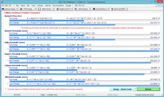
Figure POC-2 is a comparison of the different popular Turn formulae displaying the results for both a simple turn and a lane change for the given lateral distance and the inputs shown in Figure POC-1.

The assumption for all of these basic computations is that the vehicle maintains a constant velocity throughout the maneuver. The REC-TEC formulae assume an instantaneous change of direction for both the turn and the lane change maneuver, leaving it to the reconstruction expert to determine any delay in the change of direction based on human and mechanical performance during the actual maneuver in question. The other formulae use a constant that in some cases may be imputing a correction factor for the time (or distance) required to change directions over the range of actual inputs that the formula must accommodate.

POC1 shows REC-TEC generating a radius of 480.9937 ft. for the circle it uses as the model in these computations. The diameter of the circle is Radius * 2 or 961.9874 feet. This results in a circle with a circumference of 3022.1725 feet.

Figure POC-3

POC-3 shows REC-TEC generating the same radius of 480.9937 ft. for the circle it uses as the model in these computations even though the Lateral Distance has been changed to equal this radius. The diameter of the circle remains the result of the Radius * 2 or 961.9874 feet and with the same circumference of 3022.1725 feet determined by Pi * Diameter.

REC-TEC generates a subtended angle of 89.9999 for the Arc based on the 4 decimal place input for the lateral distance, as it should if modeled on a circular path. It shows a travel distance along the arc of 755.5431 feet. 755.5431 ft * 4 is 3022.1724 ft – certainly within round-off error of the calculated circumference of the circle.

If the distance of 755.5431 feet is divided by 88 f/s the result is 8.5857 seconds, the same as the Time computed for the Arc travel time in POC-3.

Figure POC-4

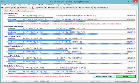
Figure POC-4 is a comparison of the different popular Turn formulae displaying the results for both a simple turn and a lane change for the given lateral distance and the inputs shown in Figure POC-3.

Suggested Further Reading: THE PROBLEM WITH TURNS Copyright © George M. Bonnett, J.D. 2001 All rights reserved. This article is contained in ANATOMY OF THE COLLISION published by IPTM, Jacksonville, FL. 1-904-620-4786 (Publication Department) or online at http://www.iptm.org.

Module 14: Fall - Vault – Airborne

(Table of Contents)

Overview: This module computes the Fall/Vault Speed (along with ancillary information) for specific input data regarding the horizontal and vertical change in the center of gravity of a vehicle (object).

At the REC-TEC pull down menu, select Fall - Vault > Airborne and the Fall - Vault – Airborne screen appears (Figure 139).

Figure 139

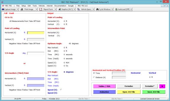
Required Inputs:

CG to CG – All measurements from Take-Off Point

Point of Landing

· Horizontal (X) – required

· Vertical (Y) – required (Negative Value if below Take-Off Point)

AND

T/O Angle – not required (default is zero)

OR

Intermediate (Third) Point

· Horizontal (X) – Measured from T/O Point

· Vertical (Y) – Measured from T/O Point (Negative Value if below Take-Off Point)

Example 1: A vehicle enters a vault landing 100 feet from and 5 feet below the point of takeoff.

What is the computed optimum angle for this vault?

What is the maximum vertical height of the vault?

What is the distance at which the vehicle reached the maximum vertical height?

What is the time at which the vehicle reached the maximum vertical height?

What is the time of the vault?

What speed the vehicle when it enters the vault?

Figure 140

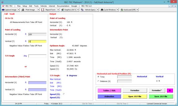
Example 2: How would the answers change with a 45-degree take-off angle?

Figure 141

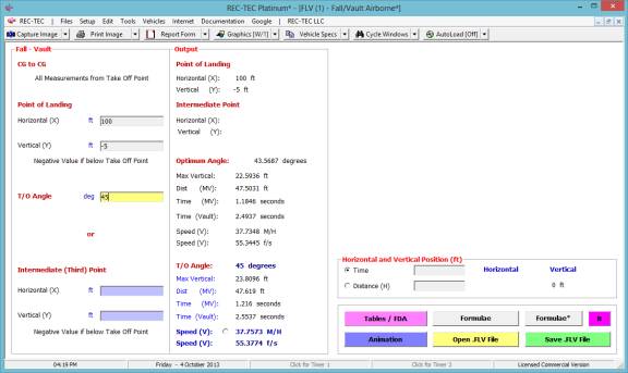
Example 3: How would the answers change with an intermediate (Third) point defined by 40 feet horizontal and (positive) 20 feet vertical?

What is the take-off angle with this third point?

Is it possible to have a different angle with a third point?

Figure 142

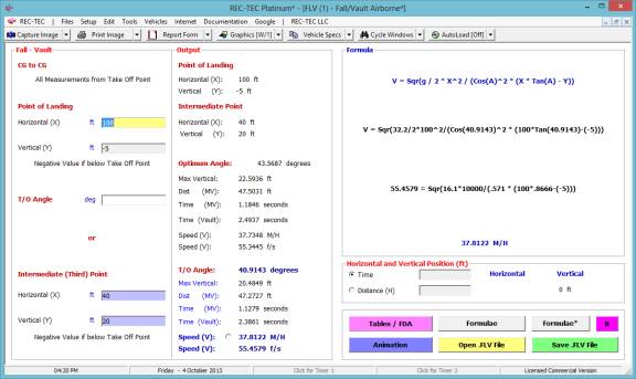
Figure 143

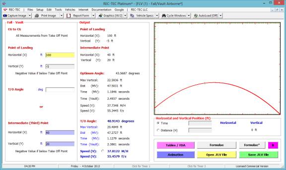
Note: Press the Formulae* button to show Figure 142. The vault is drawn to scale on both axes (Figure 143). The circle on the vault line is the third point on the vault. With a ballistic vault and three defined points on the vault, there is only one possible launch angle.

Example 4: With the same horizontal and vertical information, use a take off angle of 20 degrees.

What is the vertical and horizontal distance of the CG at 1 second into the vault?

Figure 144

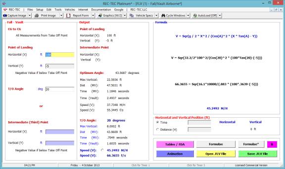
Figure 145

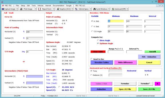
Figure 145 displays the Iteration/FDA menu. The menu includes the option of using the Optimum angle or the Given (or computed) angle. Figure 146 displays a table based on the vertical distance. The minimum is –7 and the maximum –3. The computations will be based on the given angle of 20 degrees.

Figure 146

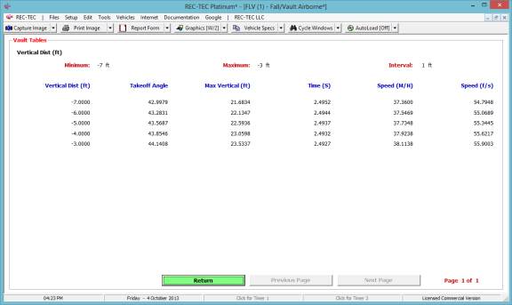
Figure 147

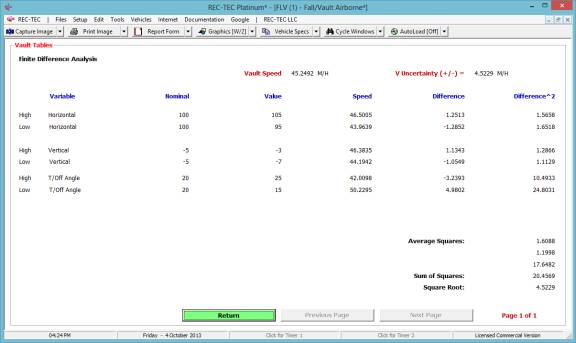
Figure 147 shows the Finite Difference Analysis using the data in Figure 145. The Uncertainty for the ranges is +/- 4.5229 M/H.

Figure 148

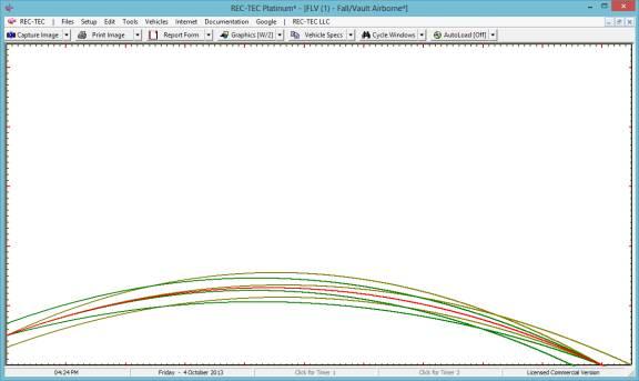
Example 5: Using a horizontal distance of 100 feet and a vertical distance of zero, what is the optimum angle and what is the resultant vault speed?

Figure 149

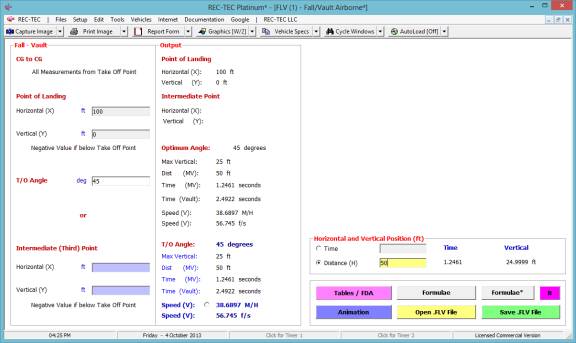
Module 15: Fall - Vault – Pedestrian-Cyclist Vault II

(Table of Contents)

Overview: This module computes the Vault Speed for Pedestrians using common formulae.

In May of 2017, Pedestrian-Cyclist Vault II was released. This is an expanded and enhanced variant of the original Pedestrian Vault.

While similar to the older variant, it has some exciting new features, which will be discussed before going into the older version.

Pedestrian-Cyclist Vault II

Figure 150-N1

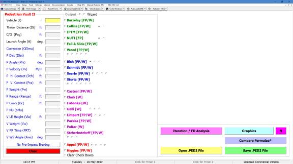
This opening screen, with no data (AutoLoad Off or after clicking on Clear) may not seem to be very helpful at first glance, but is actually a nearly perfect tool to assist with Pedestrian-Bike vaults. Print it and take it along for the next pedestrian incident. It is a list of everything the program needs for handling a pedestrian or bike vault, and will even give you a space for notes and small drawings all on one sheet.

Older users will notice that it now contains more authors (20 total) with 40 different vault formulae available to cover various situations. Many authors have multiple formulae, selected using the “Radio Buttons” after or under the name of the author. All of these buttons have ToolTips that describe what each button offers from these authors. ToolTips are also available for the Variables listed in the left hand column.

Wizard (On/Off), Defaults to On, and Clear Check Box buttons are also available.

Figure 150-N2

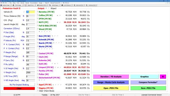
With the Wizard On and Data loaded, some of the Speeds will be in Bold Red. This is an indication that the author’s configuration for his formula is being violated by the current Inputs.

Figure 150-N3

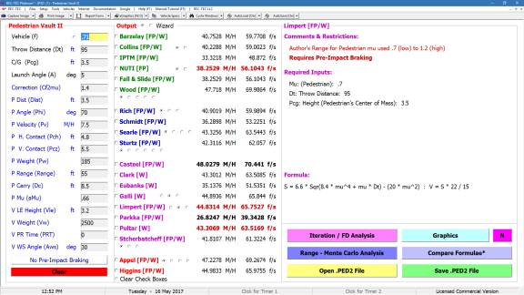
Clicking on the line for Limpert, with bold, red speeds brings up the Details Window, it states that this formula requires Pre-Impact Braking, but in the Inputs column it states that there is “No Pre-Impact Braking.” Several options are available.

Figure 150-N4

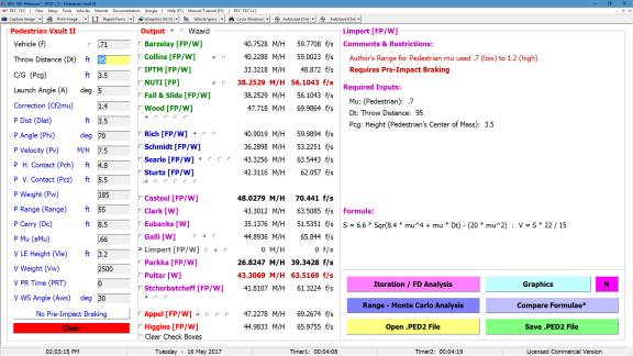
One way to remove the red speeds is to Check the box in front of Limpert. This removes this formula from all computations, including Graphics, Formulae Comparison, Iteration, Finite Difference Analysis, and Monte Carlo Analysis.

Figure 150-N5

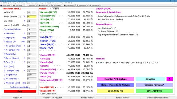
Turning the Wizard Off is another way to remove the red speeds from Limpert.

Figure 150-N6

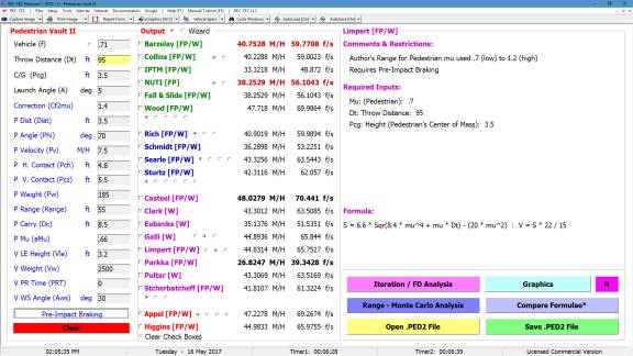
Turning ON Pre-Impact Braking will turn off the Red for Limpert, but it turns it on for

Barezlay and NUTI.

Of course you could always just ignore it.

Figure 150-N7

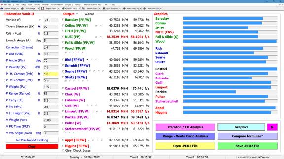
The Graphics button turns on the Graphics displaying the relative Speeds of the various Formulae chosen using the Radio Buttons.

Figure 150-N8

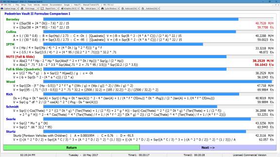
Formulae Comparison shows the relative speeds, primary and secondary speeds, the formula used to generate the speeds, and some show formula with current values.

Figure 150-N9

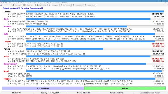
Note: Authors are arranged alphabetically within their color-coded groups. Group 1 (green), are formulae that use only the four primary Variables (black). Group 2 (blue), are four with very complex formula some using Quadratic equations.

Each grouping, except the last, ends with an author requiring multiple radio buttons that are shown below the names as they would run over the Speeds if not handled this way. There really is a method.

Figure 150-N10

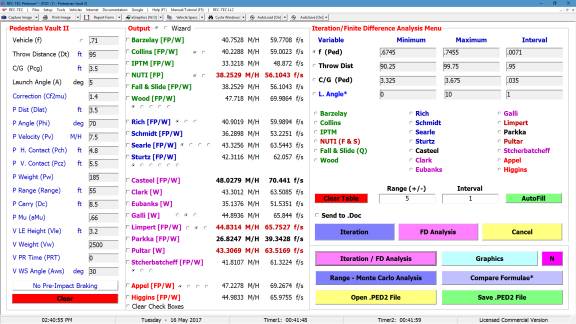
The Iteration/Finite Difference Analysis Interface shows all of the authors. AutoFill was automatically used to preset the Variables used for both Iteration and Finite Difference Analysis.

Figure 150-N11

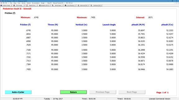
Dr. Bruno Schmidt’s formula was selected to show an example of Iteration and Jerry Eubanks’ formula was chosen to show Finite Difference.

Figure 150-N12

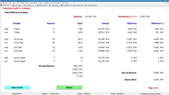
Auto~Cycler, which appears in both Iteration and Finite Difference Analysis, has 2 different functions. In Iteration it cycles the Variables, and in FDA it cycles the authors.

Figure 150-N13

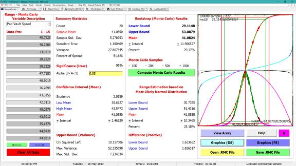
We had all 20 authors to volunteer go to Monte Carlo.

Pedestrian Fault (Original)

At the REC-TEC pull down menu, select Fall - Vault > Pedestrian (Common Formulae) and the Fall - Vault – Pedestrian (Common Formulae) screen appears (Figure 150).

Figure 150

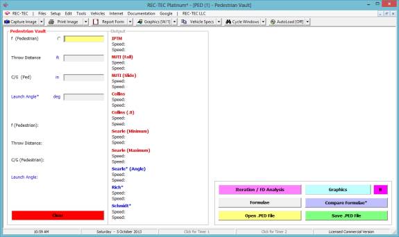
Required Inputs:

CG to CG – All measurements from Separation Point

· f (Pedestrian) – required (friction (f) between Pedestrian and Surface)

· Throw (X) – required (Separation to Point of Rest)

· C/G (Ped) – required (Center of Gravity of Pedestrian)

· Launch Angle – (Required for Searle (Angle), Rich and Schmidt formulae)

Example 1: A pedestrian comes to rest 125 feet from the point of separation with the vehicle. The coefficient of friction for the pedestrian is determined to be 0.75. The CG of the pedestrian is 2.5 feet. The launch angle for the pedestrian is 7.5 degrees.

What is the launch speed for the pedestrian?

If the information is identical, why is there a difference in the computed speeds for the different formulae?

Figure 151

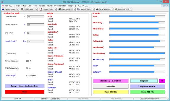
Figure 152 shows a comparison of the formulae used in this module and a graphical representation of the difference in the speeds computed for the pedestrian. Note that the Searle (Angle), Rich and Schmidt formulae utilize the launch angle as part of the computations. The other formulae assume a launch angle, but many do not state what angle is assumed in the computation.

Figure 152

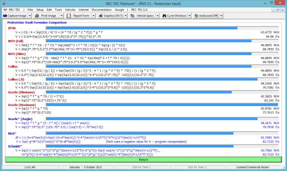
Figure 153

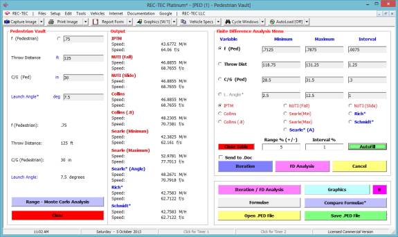
Figure 153 displays the Iteration/Finite Difference Analysis menu. The user must choose which specific formula is to be used for either, the table or, for the Finite Difference Analysis. Figure 154 will display a table for the coefficient of friction for the Searle (minimum) formula.

Figure 154

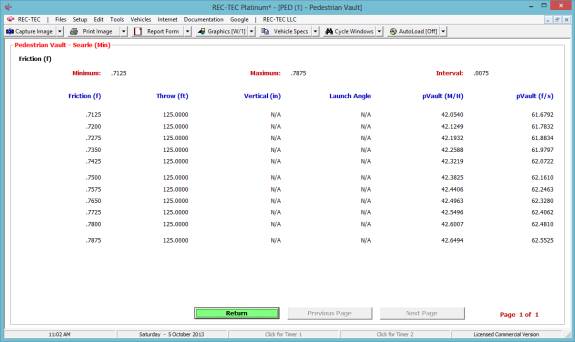
Figure 155 will show a Finite Difference analysis using the Rich formula based on the ranges specified in Figure 153 showing the base value and the uncertainty level for the given ranges.

Figure 155

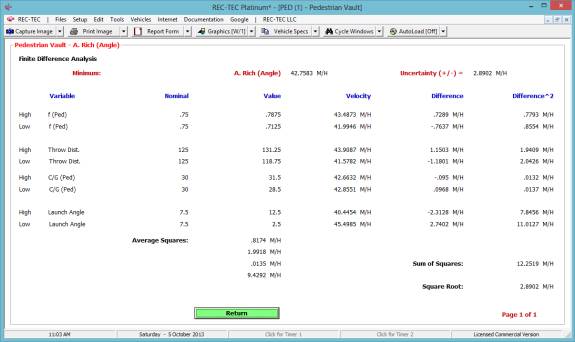
Example 2: Change the launch angle to zero with all other inputs unchanged.

Figure 156

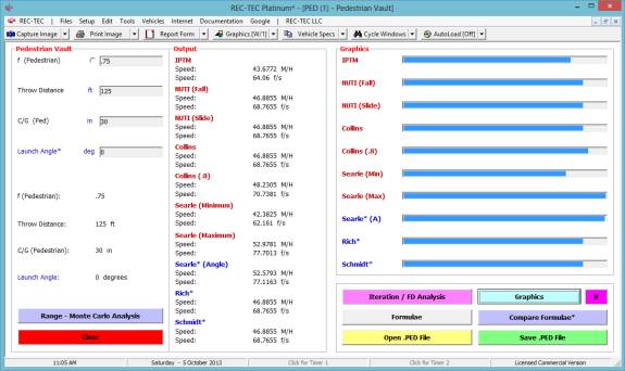
Five out of the ten formulae generate the same answer. Rich and Schmidt use the angle in their computations. This would indicate that the other three formulae with the same answer are imputing a zero-degree launch angle into the computation.

Module 16 (Vault/Slide Integration) computes the same basic answers as Rich and Schmidt.

Module 16: Fall - Vault – Vault/Slide Integration (Ped/Bike/MC)

(Table of Contents)

Overview: This module computes the Pedestrian Vault and Slide information including detailed vault data for a given throw distance, vertical change of CG, friction value and known or optimum launch angle. It will also compute a solution Launch Angle for a given speed.

Many Pedestrian Vault formulae do not allow the user to input a Launch Angle. Most of these formulae impute a launch angle using a constant within the formulae. This enhanced (2011) module will take their computed speed and compute a launch angle that generates the same speed given the same friction value, horizontal, and vertical distances.

Caution: There may be more than one solution angle for any given speed. This function will try to find the solution above the Optimum Angle (High) and the one below the Optimum Angle (Low) for the input Speed. The module also can be used in manual mode to search for other solutions.

Suggested Reading: PEDESTRIAN VAULTS – HUMANS GOING BALLISTIC by George M. Bonnett, available from IPTM. This booklet gives detailed instructions for doing this computation using four basic formulae found in any physics book.

At the REC-TEC pull down menu, select Fall - Vault > Vault/Slide Integration (Ped/Bike/MC) and the Fall - Vault – Vault/Slide Integration (Ped/Bike/MC) screen appears (Figure 157).

Figure 157

Required Inputs:

CG to CG – All measurements from Separation Point

Separation to Point of Rest

· Throw (X) – required

Separation to Point of Landing

· Vertical (Y) – required (Negative Value if below Take-Off Point)

Additional Entries

· Friction Factor – required Friction (f) between Pedestrian and Surface

· Launch Angle – (Enter if known or Click for Optimum Launch Angle)

· Command Button for Optimum Launch Angle

Optional Entry – Use to compute f for Skid

· Vault Speed – Enter Vault Speed then Click Command Button to compute Friction Factor

Example 1: A pedestrian comes to rest 125 feet from the point of separation with the vehicle. The coefficient of friction for the pedestrian is determined to be 0.75. The CG of the pedestrian is 2.5 feet. The launch angle for the pedestrian is 7.5 degrees. (Same as Example 1 in Module 15)

What is the launch speed for the pedestrian?

How far does the pedestrian slide?

How does it differ from the Rich and Schmidt solutions in Figure 151?

Figure 158

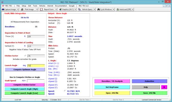
Figure 159

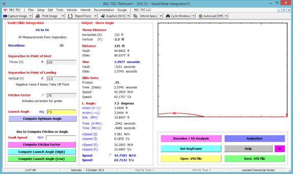
Figure 160 shows the Iteration/Finite Difference Analysis menu. The same ranges are used as in Figure 151 (Module 15).

Figure 160

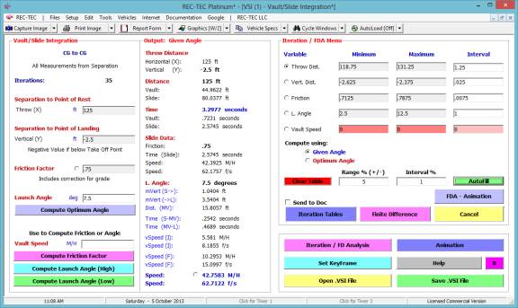
Figure 161

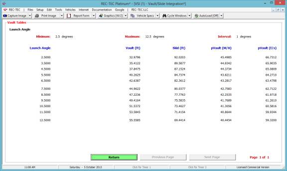
The Finite Difference Analysis solution in Figure 162 is identical to the solution in Figure 155 - (Module 15).

Figure 162

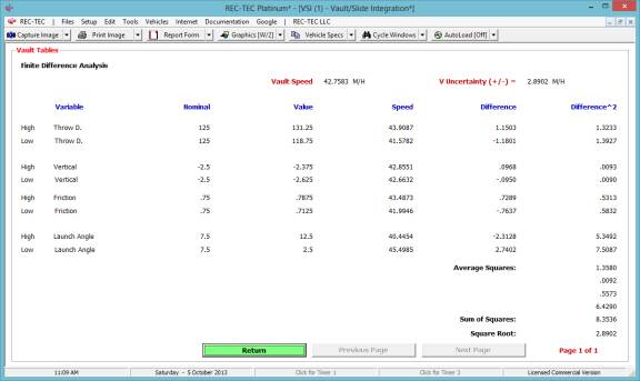
Figure 163 shows all of the vault curves and the slides for the ranges in the Finite Difference Analysis solution.

Figure 163

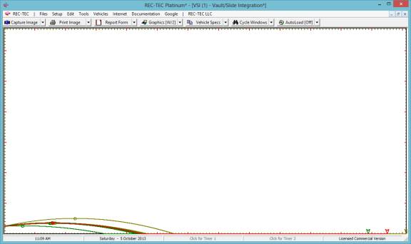
Example 2: Using the same basic information as in Figure 158, compute the optimum launch angle.

What is the optimum angle?

What is the launch speed using the optimum angle?

Figure 164

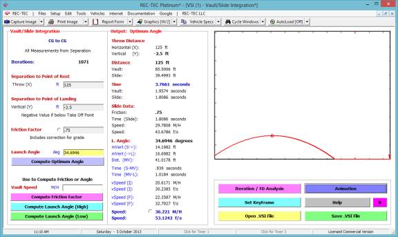
Example 3: Compute the friction value necessary for a 40 M/H vault speed using 34.6946 as the angle.

Figure 165

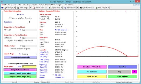
Example 4: Compute Launch Angle (High) necessary for a 40 M/H vault speed with a .75 Friction value.

Figure 165B

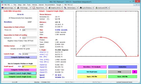
Example 5: Compute Launch Angle (Low) necessary for a 40 M/H vault speed with a .75 Friction value.

Figure 165C

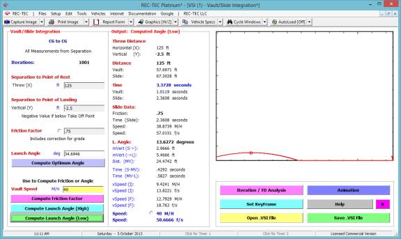
Example 6: Compute Launch Angle (High) necessary for a 45 M/H vault speed with a .75 Friction value.

Figure 165D

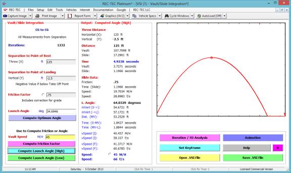
Example 7: Compute Launch Angle (Low) necessary for a 45 M/H vault speed with a .75 Friction value.

Figure 165E

Module 17: Yaw – Critical Speed – Critical Speed of Curve – Yaw

(Table of Contents)

Overview: This module computes the Yaw - Critical Speed of Curve from Friction and Chord / Middle Ordinate or Radius information.

At the REC-TEC pull down menu, select Yaw – Critical Speed > Critical Speed of Curve - Yaw and the Yaw – Critical Speed > Critical Speed of Curve - Yaw screen appears (Figure 166).

Figure 166

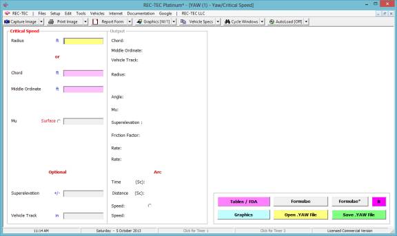
Required Inputs:

· Radius – Radius of Curve

OR

· Chord – Required with Middle Ordinate

· Middle Ordinate – Required with Chord

Required

· Mu – Surface Friction

Optional

· Superelevation – Tangent of Angle (Adjustment in direction of Striation Marks)

· Vehicle Track – Optional

Example 1: A vehicle enters a yaw on a surface that has a 0.65 coefficient of friction. A measured 50-foot chord has a 36-inch middle ordinate.

What is the average speed for the yaw?

What is the radius of the yaw?

Figure 167

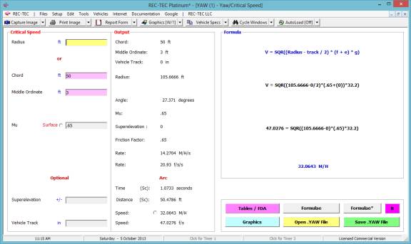
Figure 168 shows a graphic of the event as part of the circle having the computed radius. Figures 167 and 168 show the results of using chord and middle ordinate computations.

Figure 168

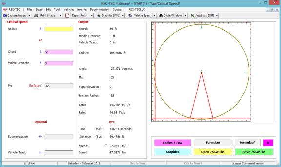
Example 2: A vehicle enters a yaw on a surface that has a 0.65 coefficient of friction. The radius was determined to be 105 feet.

What is the average speed for the yaw?

Figure 169

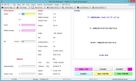
Figure 170

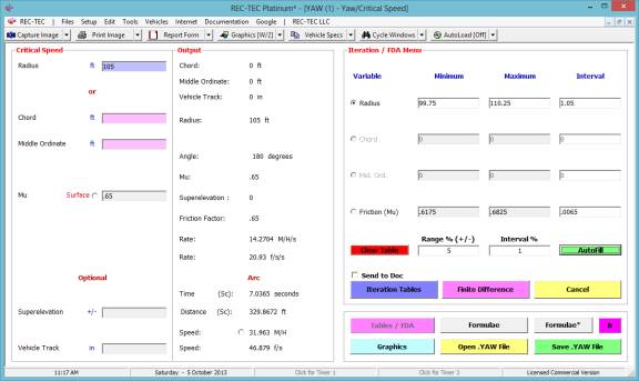
Figure 170 displays the Iteration/Finite Difference Analysis menu. There is no provision for varying the Superelevation or the Vehicle Track. Both of these variables can be accommodated using the either, the radius, or the surface friction.

Figure 171 shows the iteration of the surface friction and the resulting computed average speed for the yaw. The distance computed is for the half circle (0.5 * circumference) with the given radius.

Figure 171

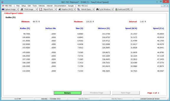
Figure 172 displays the results of the Finite Difference Analysis using the ranges for the variables in Figure 170.

Figure 172

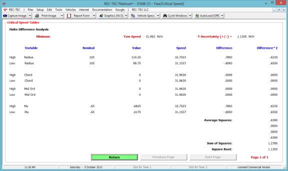
Example 3: A vehicle enters a yaw on a surface that has a 0.65 coefficient of friction. A measured 50-foot chord has a 36-inch middle ordinate. The track of the vehicle is 60 inches and the Superelevation is +0.05.

Figure 173

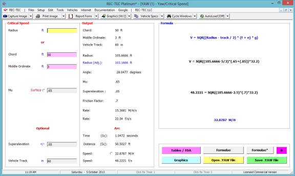
Figure 174 shows the Finite Difference Analysis ranges of the Chord and Middle Ordinate.

Figure 174

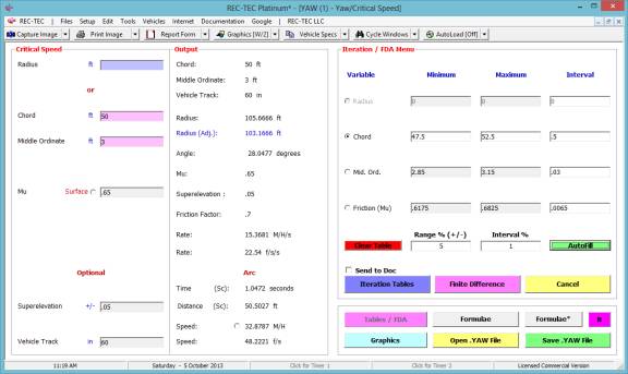
Figure 175 shows the results of the Finite Difference Analysis using the Chord and Middle Ordinate computations.

Figure 175

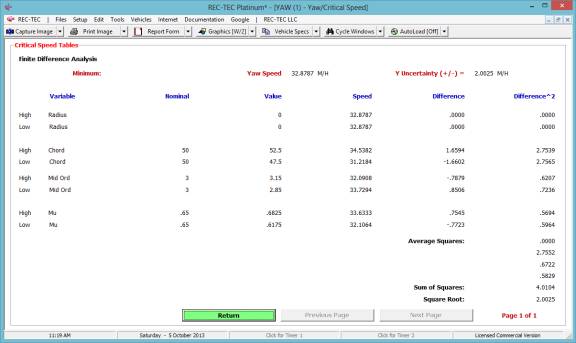
Question 2 in this module asked about the Radius of the circle. See Figure 167 for the results. Now look at Figure 176. It is a Time - Distance Single Surface Deceleration using the average speed of the yaw as the initial speed. Can you spot the relationship?

Figure 176

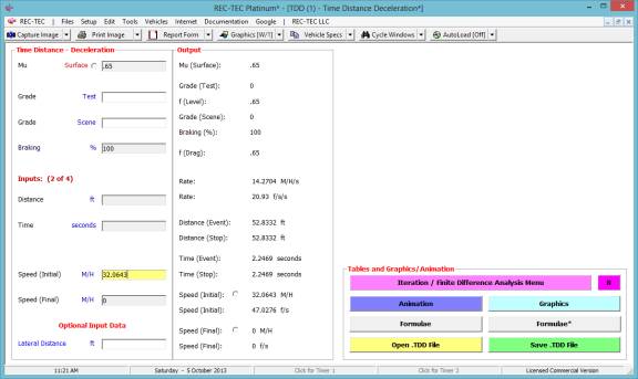
Hint: Look at the distance necessary for decelerating to a stop.

Module 18: Time - Distance – Motion Analysis

(Table of Contents) (Table of Contents)

Overview: This module computes speed dissipation from wheel forces due to position. It can be used for spins, yaws or decelerations. This module can be used for either a Critical Speed Maneuver or a Spin. Analysis is by position (Work-Energy computation).

At the REC-TEC pull down menu, select Time - Distance > Motion Analysis (1-99 Phases) and the Motion Analysis screen appears (Figure 177).

Figure 177

Required Input Data

Data Entry:

Common:

· Number of Phases

· Mu (Deceleration) - Baseline Surface Friction for all Phases

· Rolling Resistance - Baseline Rolling Resistance for all Phases

· Final Speed

· Front Weight %

· Initial Slip Angle

· KeyFrame/Time – Not Required. Entering KeyFrame shows start time for Animation Output files (Hi-Resolution Animation).

Phase Inputs

· Phase (Current Phase of Total Number of Phases) - Click Up/Down Arrow to Change phase

· Mu (Phase Adjustment to Baseline Surface Friction – Includes change due to Grade for 3D)

· Rolling Resistance (Phase Adjustment to Baseline Rolling Resistance)

Datum Line / Distance

· Linear (Phase only)

· Offset (Total)

· Vehicle Airborne (Phase) check block - Object will not decelerate during this phase if checked

· Z-Axis Height - Elevation of Road Surface (Z-Axis Height) over which vehicle is traveling – The Surface Friction (Mu) must be adjusted for change in Grade.

· Final Slip Angle (Phase)

Slip Angle Adjustments (Degrees)

· Left Rear

· Left Front

· Right Front

· Right Rear

Percent of Braking (0 to 100)

· Left Rear (0 to 100)

· Left Front (0 to 100)

· Right Front (0 to 100)

· Right Rear (0 to 100)

Example 1: The inputs for even a small yawing type maneuver can be cumbersome. In an effort to save time, the inputs will not be shown for this problem as they are duplicated on the output screen. The file being used is named Problem19.SPN.

Figure 178

Figure 179 displays the warning that Time - Distance Motion Analysis operates in the same direction as the arrow of time.

Figure 179

Figure 180 displays the animation of the vehicle over the points input into the different phases computing the resulting values for time and speed based on position-based deceleration.

Figure 180

Full screen animation is activated by using the [Esc]ape key when the smaller animation frame is displayed.

Figure 181

Figure 181 shows the Data Table. This table includes the inputs and computed data resulting from these inputs. The Table headings are explained below.

Table Legend

· # – Phase Number

· Dist – Distance Parallel to Datum Line (Phase Only)

· Dist – Distance Parallel to Datum Line (Cumulative)

· Dist – Distance Traveled by Center of Mass (Phase Only)

· Dist – Distance Traveled by Center of Mass (Cumulative)

· Offset – Distance Perpendicular to Datum Line

· Time – Phase

· Time – Cumulative

· VSA – Vehicle Slip Angle (Average)

· LR – Left Rear Adjustment (Right = Positive | Left = Negative)

· LF – Left Front Adjustment (Right = Positive | Left = Negative)

· RF – Right Front Adjustment (Right = Positive | Left = Negative)

· RR – Right Rear Adjustment (Right = Positive | Left = Negative)

· f(T) – Total Drag Factor (Vehicle)

· LR – Left Rear – Drag Factor

· LF – Left Front – Drag Factor

· RF – Right Front – Drag Factor

· RR – Right Rear – Drag Factor

· Speed – Speed (Primary)

· Speed – Speed (Secondary)

Example 2: A vehicle skids over 3 surfaces to a stop. The vehicle has 100% braking throughout the skid. There is no grade.  

1. Surface #1: .75 drag factor 43 feet

2. Surface #2: .6 drag factor 27 feet

3. Surface #3: .25 drag factor 52 feet to a stop

Figure 182

Figure 182 shows the initial entry (last phase of the deceleration), which in this case goes to zero.

Figure 183

Figure 183 shows the second entry (middle phase of the three-phase deceleration).

Figure 184

Figure 184 shows the third entry (first phase of the deceleration).

Figure 185

Figure 185 shows the data table for all three events. The top line shows the initial speed for the maneuver.

Figure 186

Figure 186 displays the animation for all three phases of the maneuver.

Figure 187

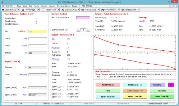
Figure 187 shows the same problem (Example 2) run in Time - Distance Multiple Surfaces. This solution is identical to the solution in Motion Analysis and shows the deceleration curves.

Module 19: Yaw - Critical Speed – Motorcycle Lean Angle

(Table of Contents)

Overview: This module computes the Radius, Speed, Lean Angle and/or Friction Factor for (2-wheeled) motorcycles or bicycles in a turn.

At the REC-TEC pull down menu, select Yaw - Critical Speed > Motorcycle Lean Angle and the Motorcycle Lean Angle screen appears (Figure 188).

Figure 188

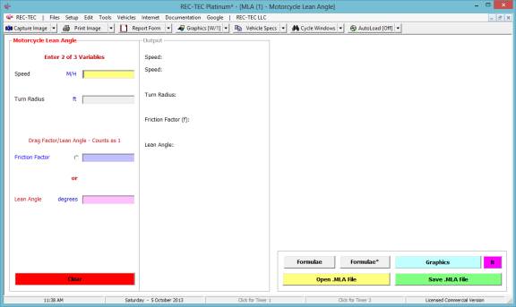
Required Input Data

This module contains four data entry blocks. Two of the four are required. Friction Factor or Lean Angle may be entered, but not both.

· Speed – Speed of Vehicle entering Curve

· Turn Radius – Radius of Curve

· Friction Factor – Adjusted for Grade and Superelevation

· Lean Angle – Actual or Maximum

Example 1: A motorcycle is traveling at 60 M/H on a surface with a .75 coefficient of friction and enters a turn.

What is the turn radius?

What is the lean angle?

Example 2: A motorcycle enters a turn with a lean angle of 17.5 degrees and a turn radius of 45 feet.

What is the friction factor?

What is the speed of the bike?

The solution to Example 1 is shown in Figure 189.

Figure 189

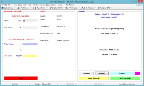
The solution to Example 2 is shown in Figure 190.

Figure 190

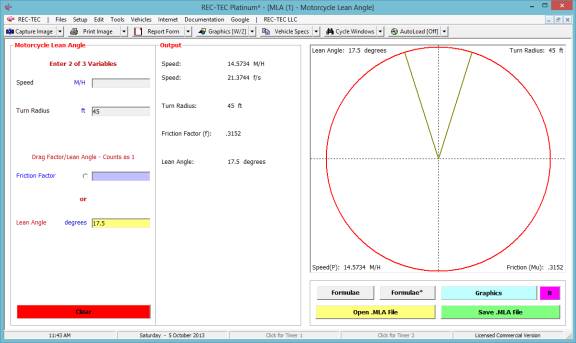
Module 20: Energy – Conservation of Energy

(Table of Contents)

Overview: This module computes for unknowns in the collision using Conservation of Energy.

At the REC-TEC pull down menu, select Energy > Conservation of Energy and the Conservation of Energy screen appears (Figure 191).

Figure 191

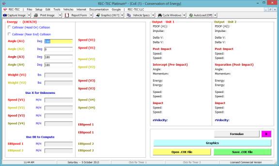
Required Input Data

· Checkbox for Collinear (Head On) Collision – Check if Collinear Head-On Collision

· Checkbox for Collinear (Rear End) Collision – Check if Collinear Rear-End Collision

Angles (Enter appropriate angle for Left/Right Hand Coordinate System & Heading/Radial configuration)

· Angle (A1) – Approach Angle for Unit 1

· Angle (A2) – Approach Angle for Unit 2

· Angle (A3) – Departure Angle for Unit 1

· Angle (A4) – Departure Angle for Unit 2

Weights

· Weight (V1) – Weight of Unit 1

· Weight (V2) – Weight of Unit 2

Speeds (2 Unknowns Allowed)

· Speed (V1) – Approach Speed of Unit 1 – Use X if Unknown

· Speed (V2) – Approach Speed of Unit 2 – Use X if Unknown

· Speed (V3) – Departure Speed of Unit 1 – Use X if Unknown

· Speed (V4) – Departure Speed of Unit 2 – Use X if Unknown

Equivalent Barrier Speeds (1 Unknown allowed)

· EBSpeed 1 – Equivalent Barrier Speed of Unit 1 – Use X if Unknown

· EBSpeed 2 – Equivalent Barrier Speed of Unit 2 – Use X if Unknown

Example 1: Vehicle #1 (3129#) is traveling eastbound when it is struck by Vehicle #2 (3375#) traveling westbound. Both vehicles stop at impact. Vehicle #1 has an EBS from CRUSH of 48 M/H and Vehicle #2 has an EBS of 48.2 M/H.

Figure 192

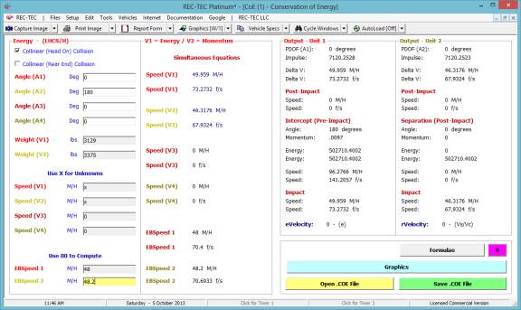
Figure193

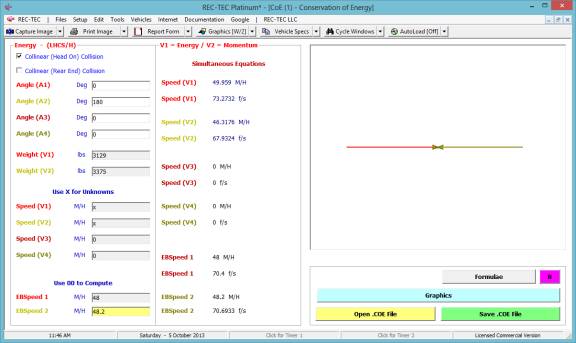
The unknowns in Example 1 are the impact speeds for Vehicle 1 and Vehicle 2. The module uses two simultaneous equations to arrive at a solution (Figures 192 and 193).

Example 2: Vehicle #1 (3070#) is traveling eastbound when it strikes Vehicle #2 (3205#) which is stopped. Vehicle #1 has a post impact speed of 16.4 M/H and an EBS from CRUSH of 12.8 M/H. Vehicle #2 has a post impact speed of 16.6 M/H and an EBS of 16.5 M/H.

Figure 194

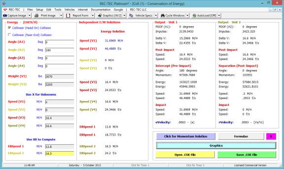
Figure 195

The unknown in Example 2 is the impact speed for Vehicle 1. The module arrives at an Energy solution in Figures 194 and 195.

Figure 196

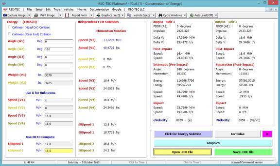
Figure 197

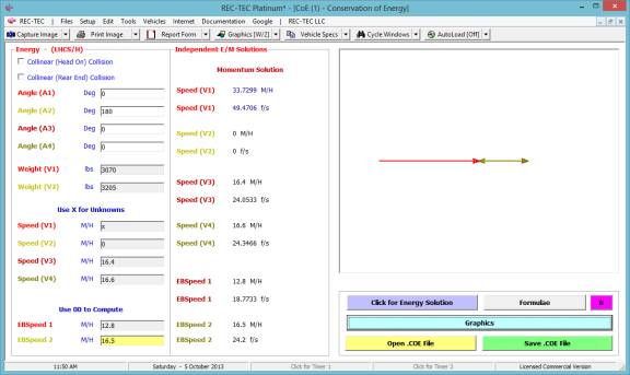
The unknown in Example 2 is the impact speed for Vehicle 1. The module arrives at a Momentum solution in Figures 196 and 197. Compare this with the Energy solution in Figures 194 and 195.

Example 3: Vehicle #1 (3275#) is heading towards 0 degrees when it is struck by Vehicle #2 (3500#) approaching from 170 degrees. Vehicle #1 departs at an angle of 343 degrees at 10.4 M/H and Vehicle #2 departs at an angle of 50 degrees at 9.9 M/H. Vehicle #1 has an EBS from CRUSH of 38.3 M/H and Vehicle #2 has an EBS of 41.2 M/H.

Figure 198

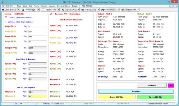
Figure 199

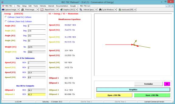
The unknowns in Example 3 are the impact speeds for Vehicle 1 and Vehicle 2. The module uses two simultaneous equations to arrive at a solution (Figures 198 and 199).

Example 4: Re-run Example 3 as a collinear head on collision.

Figure 200

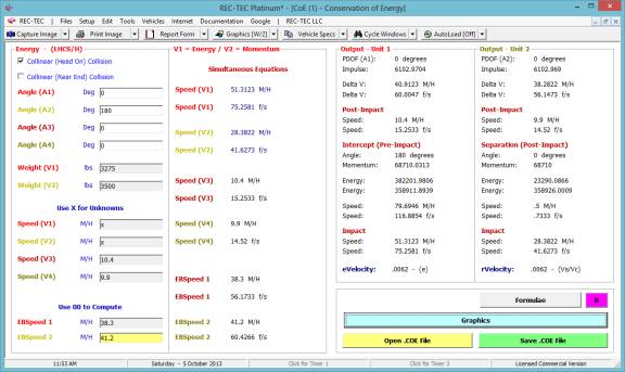
Figure 201

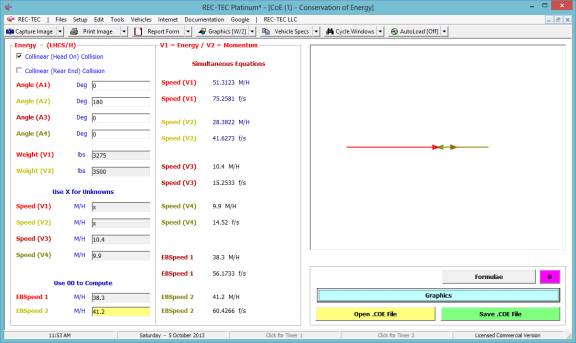
The unknowns in Example 4 are the impact speeds for Vehicle 1 and Vehicle 2. The module uses two simultaneous equations to arrive at a solution (Figures 200 and 201).

Example 5: Vehicle #1 (3850#) is traveling eastbound when it strikes Vehicle #2 (2520#) which is stopped. Both vehicles depart together at the same speed. Vehicle #1 has an EBS from CRUSH of 17.6 M/H and Vehicle #2 has an EBS of 26.0 M/H.

Figure 202

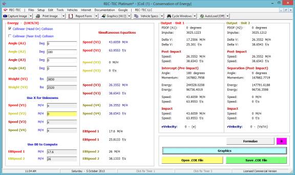
Figure 203

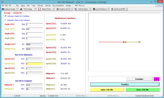
The unknowns in Example 5 are the impact speed for Vehicle 1 and the post impact speeds for Vehicle 3 and Vehicle 4. While there are three unknowns, two of them are identical and can be treated as one unknown. The module uses two simultaneous equations to arrive at a solution (Figures 202 and 203).

Module 21: Energy – Kinetic

(Table of Contents)

Overview: This module computes the unknowns in the basic Kinetic Energy formulae for complex events and displays both the energy and momentum of the object.

At the REC-TEC pull down menu, select Energy > Kinetic and the Kinetic Energy screen appears (Figure 204).

Figure 204

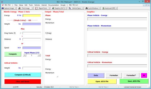
Required Input Data

· Energy – Energy value for Phase (computed independently)

(Single Entry) - - OR

· Weight – Weight of Vehicle

Plus

· Drag Factor (f) – Restitution value for the Collision

· Distance – Weight of Vehicle 1

Or

· Speed – Change of Velocity for Vehicle 1

Re-Compute (Command Button) – Allows Computation of New Data Only – Required for Further Computations.

Input Phase (max = 15) – Shows Phase as Current (Before Compute). Arrows or direct entry permits viewing earlier Phases

Critical Vehicle: – Critical Vehicle or Object

· Weight – Weight of Critical Vehicle

Compute (Critical) – Computes data for Speed based on Critical Vehicle Weight

Clear and Reset – Clears and Resets all input entry blocks

Example 1: A vehicle weighing 2000 pounds is responsible for three “packets” (Phases) of energy. The initial Phase consists of 10000 ft*lbs of energy. Phase 2 consists of moving a 2500-pound vehicle 100 feet over a surface with a drag factor of 0.7. The third Phase consists of a 3500 pound vehicle traveling at 60 M/H to a complete stop.

What was the speed of the “Critical” vehicle?

What was the total energy in this event?

Figure 205

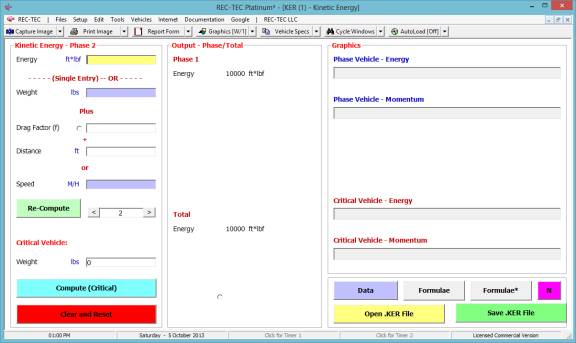
Figure 205 shows Phase 1 entry data.

Figure 206

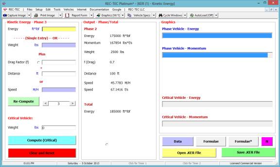
Figure 206 shows Phase 2 entry data.

Figure 207

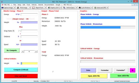
Figure 207 shows Phase 3 entry data.

Figure 208

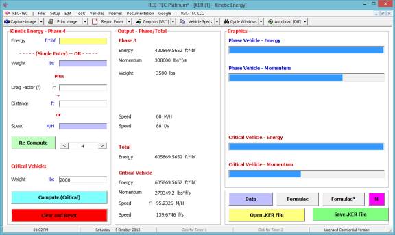
Figure 208 shows computation for Critical Vehicle solution.

Figure 209

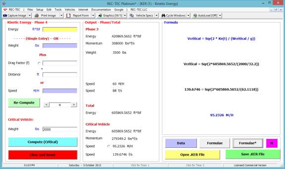
Figure 209 shows the formula for the Critical vehicle solution.

Figure 210

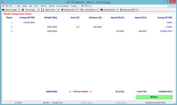
Figure 210 displays the data table with all three phases and the solution based on the weight of the Critical Vehicle.

Module 22: Energy – Break Fracture

(Table of Contents)

Overview: This module computes Energy to break a wooden pole (power pole, utility pole) based on its circumference.

At the REC-TEC pull down menu, select Energy > Break Fracture and the Break Fracture screen appears (Figure 191).

Figure 211

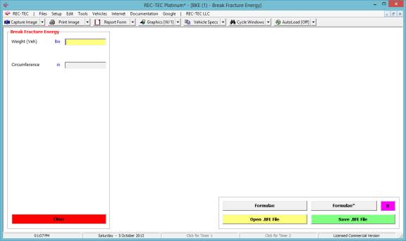
Required Input Data

· Weight (Veh) – Weight of Vehicle

· Circumference – Circumference in selected Unit of Measure

Example 1: A vehicle weighing 2795 pounds strikes a wooden utility pole with a circumference of 30 inches.

1. What is the speed required to break the pole?

2. What is the fracture energy required?

Figure 212

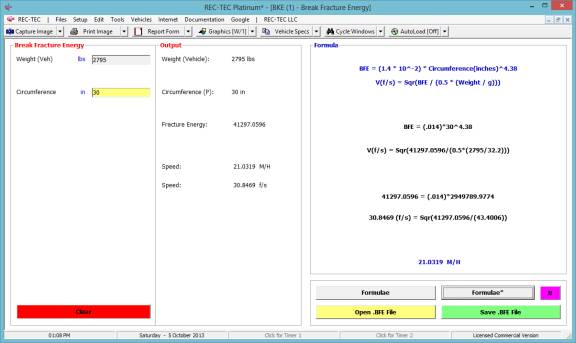
Module 23: Momentum – 360 Digital Momentum

(Table of Contents)

Overview: This module computes the Impact Speeds, Angles and DeltaVs for angular and inline collisions using a Drag and Drop interface with digital inputs available on an interactive graphical interface. This module interface effectively marries output from the CrushV module and Motion Analysis modules using a graphics display to consolidate information on position and damage analysis verifying the linear momentum solution. It then takes the finalized data and transfers it to the 360 Linear Momentum module for further technical and statistical analysis.

At the REC-TEC pull down menu, select Momentum > 360 Digital Momentum and the 360 Digital Momentum screen appears (Figure 213).

Figure 213

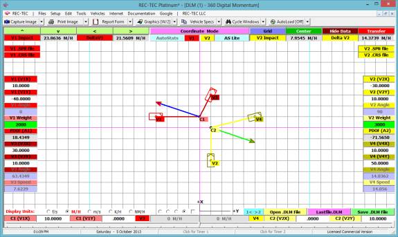
Required Input Data

Approach Data:

Angles (1 and 2) – Approach Angles are automatically computed when the “flags” for the vehicles (V1 and V2) are moved by grabbing and dragging them with the mouse or by manually entering the values for the X and Y positions of the vehicle CG.

Weights (1 and 2) – Weight, length and width of each vehicle is automatically entered if the user employs AutoStats or AutoStats Lite and selects a particular vehicle for transfer to Digital Momentum.

Collision Data:

CG Location at Collision – These points are automatically computed when the “flags” for the vehicles (C1 and C2) are moved by grabbing and dragging them with the mouse or by manually entering the values for the X and Y positions of the vehicle CG.

Departure Data:

Angles (3 and 4) – Departure Angles are automatically computed when the “flags” for the vehicles (V3 and V4) are moved by grabbing and dragging them with the mouse or by manually entering the values for the X and Y positions of the vehicle CG.

Speeds (3 and 4) – are automatically computed when the “flags” for the vehicles (V3 and V4) are moved by grabbing and dragging them with the mouse or by manually entering the values for the X and Y positions of the vehicle CG. These post-impact speeds are determined by the length of the departing vector.

Coordinate Mode: Coordinate mode allows drag-drop positioning of vehicles and collision points. It also permits direct entry of the X and Y-coordinate points of the approach angles of V1 and V2 and the velocity vectors for V3 and V4. These points determine approach angles, post-impact velocities of the vehicles and the collision points.

Analytical Mode: While coordinate mode allows direct numerical entry and manipulation of the X and Y Coordinates for approach, collision and departure, it should not be used in conjunction with the Departure data files imported from Motion Analysis. Since the Motion Analysis files represent hard data measured at the scene regarding distances, it would be improper to manipulate this data.

The departure speeds and departure angles are variable (numerical inputs - Analytical Mode) depending on the friction and braking and departure angles of the vehicles. The user is also allowed to vary the approach angles (numerical inputs - Analytical Mode) accommodating the last minute evasive action by one or both drivers. As these changes are entered, the locations of the new approach and departure vehicles are displayed as vectors scaled to the approach and departure speeds and angles.

The original locations are displayed as located by coordinate positions (not scaled to the speeds) and the heading angles of the original Approach and Departure vehicles match the new Approach and Departure vectors.

Graphics: The basic graphics display shows the pre-impact vector (angle and speed), the CG location at collision and the post-impact vector for each of the vehicles. The X and Y coordinate positions are given for each of the points described as well as the weights, speeds and angles associated with the event. The PDOF/Impulse vectors are also shown for the collision. Impact speed and DeltaV is shown for each vehicle at the top of the screen.

The center-top buttons (V1 & V2 .SPN file) will permit Motion Analysis files to be imported as post-impact trajectory data for each vehicle including the trajectory over the ground, which is drawn to scale. The AutoStats and AutoStats Lite Buttons allow importing of critical vehicle dimensional data (including weights) that is used to draw scale outlines of the vehicles.

The upper-right buttons (V1 & V2 .CRS file) will permit CrushV files to be imported with scale dimensional data as well as CrushV profiles of the damage (including C measurements and Zones) for graphical display and analytical analysis. The centroids of damage of the vehicles are displayed as well as PDOF, lever arm, Impulse vectors, and computed rotational information. The program then re-computes the PDOF and Impulse information based on the momentum data for the collision configuration and displaying these vectors in addition to that imported from CrushV allowing verification of the CrushV PDOF input data.

Example 1: Using direct entry, Enter 50 for V3-V3X and either hit the enter key or click on the V3-V3X button. Enter 20 for V3-V3Y and either hit the enter key or click on the V3-V3Y button. Enter 20 for V4-V4X and either hit the enter key or click on the V4-V4X button. Enter 50 for V4-V4Y and either hit the enter key or click on the V4-V4Y button.

1. What is the V1 impact speed?

2. What is the V3 departure angle?

3. What is the V1 DeltaV?

4. What is the V2 impact speed?

5. What is the V4 departure angle?

6. What is the V2 DeltaV?

Figure 214

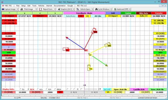
Entry must be in Coordinate mode. Press the F1 key to discover the functions of the buttons surrounding the display. The Hide Data button will remove most of the buttons and entry labels. The Grid button will remove the grid leaving only the axes.

Figure 215

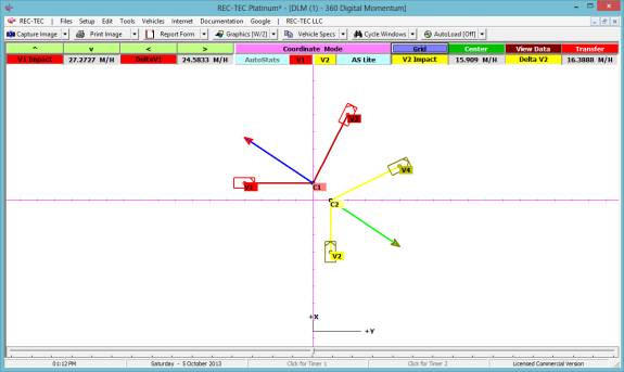
Clicking on the Transfer button will automatically transfer the data to the 360 Linear Momentum Module (Figure 216).

Figure 216

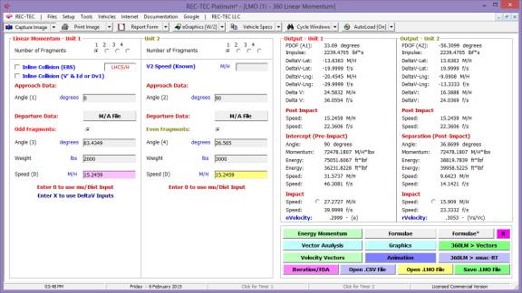
The answers shown in Figure 216 are identical to the answers in Figures 214 and 215.

Figure 217

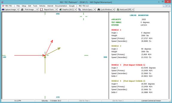
The basic graphics in Figure 217 are identical to the graphics in Figures 214 and 215. This transfer allows additional analysis capabilities not available in the Digital Momentum module.

Exit the Linear Momentum module and the Digital Momentum module reappears. Right click on the mouse and the Digital Momentum graphics are re-drawn.

Example 2: Click on View Data to recover the full functionality of the interface. Click the V1.SPN file button to load a .SPN file. Open Problem 19. Click the V2.SPN file button to load a .SPN file. Open Problem19X. Use the slider at the bottom of the screen to zoom out on the graphics.

Figure 218

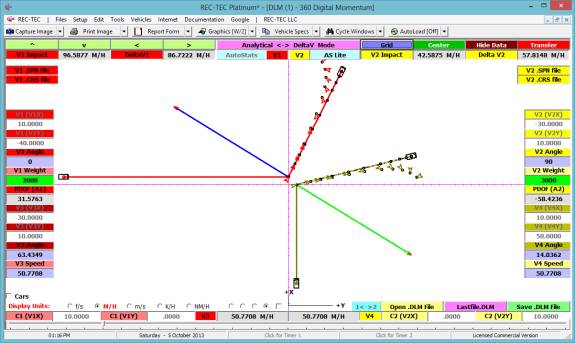
The module automatically switched to the Analytical mode. In this mode, the permissible direct entries are the four angles and the post-impact speeds. Change the angle of V3 to 45 degrees and the angle of V4 to 20 degrees

Figure 219

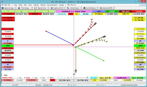
Example 3: Using the Example 2 configuration, enter 65 for the speed of V3. Look just below the V3 entry and check the Cars box. Use the arrows in the upper left of the screen to center the collision.

Figure 220

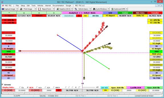
When the speed was changed for V3 on the left side of the screen, the computed speed for the loaded file remains in the V3 block in the lower center of the screen. The user cannot change that entry.

Figure 221

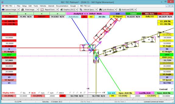
Figure 221 has Car1.CRS loaded for V1, Car1A.CRS loaded for V2 and is zoomed into the collision.

Example 4: Notice that the damage did not line up for maximum engagement. Change the angle of V2 to 50 degrees, V3 to 35 degrees, and V4 to 20 degrees.. Place a check in the Centroid box in the lower right of the screen. Now click on the Center button in the upper right corner of the screen.

What are the impact speeds of V1 and V2?

Figure 222

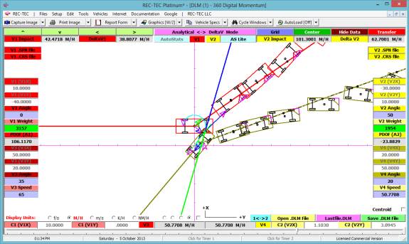
Transfer the data to Linear Momentum and compare results.

Figure 223

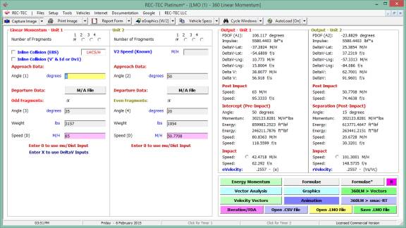
Figure 224

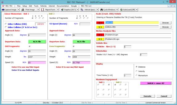
Click the Animation button. Change the Vehicle size to 5 and set the Display to Distance and set the maximum engagement as shown in Figure 224. The rest of the data was automatically transferred from Digital Momentum.

Figure 225

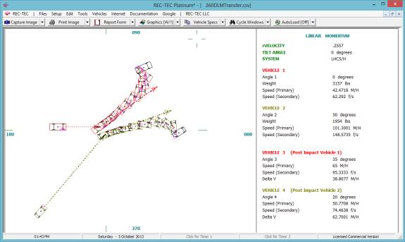
The advanced analysis options in Linear Momentum are explored in Module 24.

Example 5: Exit out of the program. Re-Enter and go to Digital Momentum with AutoLoad[On]. The file does not automatically re-load. Open “Lastfie.DLM” and the file is opened. (See Figure 226)

Figure 226

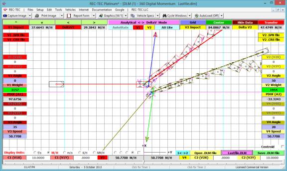
The file is opened, but the V3 and V4 speeds have been reset, the line width, which had been changed to 2 in Figure 221 is now back to 1 and the zoom has been returned to the default setting. Set the zoom to maximum and then re-center the drawing.

Figure 227

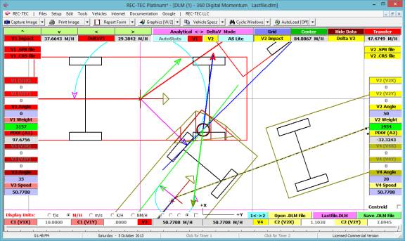
Notice that the Centroids of Damage overlap each other. The rotation directional arrows and the user entered PDOF arrows from the CRUSH module (.CRS) vehicles are displayed along with the damage profiles for each of the vehicles.

Example 6: Use the REC-TEC dropdown menu to open (another) Digital Momentum module. You may now cycle between the Windows or Tile them (Vertically) as displayed in Figure 228. In Figure 228 each Window has been re-centered.

Figure 228

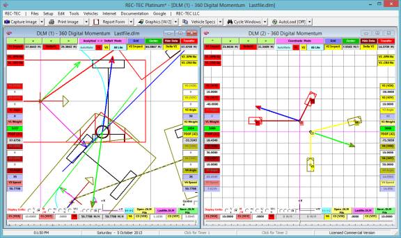
Have DLM(2) go Full screen by double right clicking on the top bar of the DLM(2) window. Left click on the screen to cause a re-draw. Click on the Autostats Lite button.

Figure 229

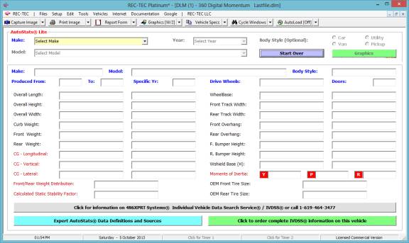
Select your vehicle and then Click on the red “Return to Digital Momentum with current data” button.

Figure 230

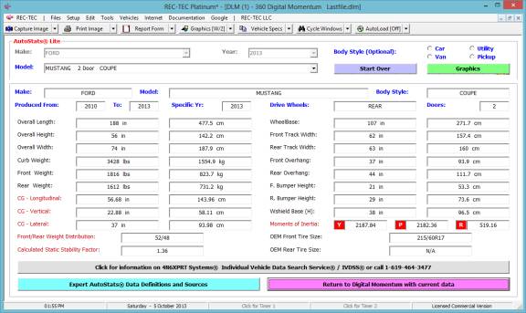
Notice the ToolTip displayed in Figure 231. Click on the V1 button to transfer the AutoStats data to V1.

Figure 231

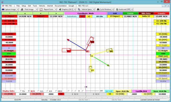
Repeat the above (AutoStats or AutoStats Lite) procedure for V2. Figure 232 will show a 2004 Hummer 4Door 4X4 Utility for Vehicle 2.

Figure 232

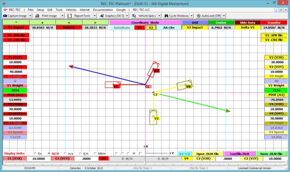
Note how the V1 and V2 Impact speeds have changed as a result of the Autostats Lite data, including the vehicle weights. Figure 232 shows the speeds in M/H and Figure 233 shows them in f/s.

Figure 233

Example 7: Grab the flags for the vehicles and collision points and move them around. Note how the PDOF (DeltaV) lines also move and change length with the changing values.

Module 24: Momentum – 360 Linear Momentum

(Table of Contents)

Overview: This module computes the Impact Speeds, DeltaVs, PDOFs, Energy and Momentum data for angular and inline collisions.

At the REC-TEC pull down menu, select Momentum > 360 Linear Momentum and the 360 Linear Momentum screen appears (Figure 234).

Figure 234

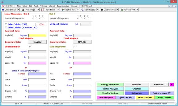
Required Input Data

Number of Fragments (1 - 4)

Program accommodates up to four exit fragments for each Entry Unit

Checkbox for Inline Collision (EBS) – Check if Rear End Collision

· Checking this box calls up a frame for entering EBSpeeds for both units if desired. The Equivalent Barrier Speeds enter into the computations for the impact speeds. If no EBS Speeds are entered, Minimum and Maximum speeds are computed for Rear End collision

V2 Speed (Known) – Enter Value in Textbox

Negates the computation of V2 and proceeds to compute V1 based on the value entered.

Checkbox for Inline Collision (V’ & Ed or Dv1) – Check if Rear End Collision

· Checking this box calls up a frame for entering known common post-impact Speed for both units. The known DeltaV1 (use +/- sign) or total Damage Energy must also be entered. This procedure computes the approach angles for the vehicles. This feature was added in November 2011 – New screen is displayed in Figure 234

This module contains the following data entry blocks for each of the two Units within the leftmost set of frames:

Approach Data:

· Angle (1 or 2) – Approach Angle (Enter appropriate angle for Left or Right Hand Coordinate System / Heading or Radial configuration)

Departure Data:

· Motion Analysis files may be used for Departure information (single fragment only). These files will supply Departure Speeds and Trajectory data for Animation.

Odd / Even Fragments:

· Angle (N) – Approach Angle (Enter appropriate angle for Left or Right Hand Coordinate System / Heading or Radial configuration)

· Weight – Entered as actual weight or ratio

· Speed – Enter Post-Impact speed or enter zero (0) to display frame for entering the following data:

Or

· Mu

· Grade (Test)

· Grade (Scene)

· % Braking (100)

· Distance

Output: The two frames on the right side of the screen show the Output – Unit (1 or 2) information as follows:

· PDOF(A-Number) – Direction of Impulse Vector relative to heading of Vehicle

· Impulse: Change of Momentum

· DeltaV-Lat: Lateral Change of Velocity (Primary)

· DeltaV-Lat: Lateral Change of Velocity (Secondary)

· DeltaV-Lng: Longitudinal Change of Velocity (Primary)

· DeltaV-Lng: Longitudinal Change of Velocity (Secondary)

· DeltaV: Change of Velocity (Primary)

· DeltaV: Change of Velocity (Secondary)

Post Impact

· Speed: Impact Speed (Primary) – Input or Computed

· Speed: Impact Speed (Secondary) – Input or Computed

Intercept (Pre-Impact) and Separation (Post-Impact)

· Angle: Intercept (Closure) / Separation

· Momentum: Pre-Impact / Post-Impact

· Energy: Kinetic at Impact / Kinetic after Impact

· Energy: Actual / Maximum for Damage including Rotation

· Speed: Speed (Primary) – Closure / Separation

· Speed: Speed (Secondary) – Closure / Separation

Impact

· Speed: Impact Speed (Primary)

· Speed: Impact Speed (Secondary)

eVelocity: Coefficient of Restored System Velocity (Restitution)

rVelocity: Coefficient of Retained System Velocity (Vs/Vc)

Example 1: Vehicle 1 (2000#) traveling due east collides with Vehicle 2 (3000#) traveling due north. V1 exits at 30 degrees to the east of due north and a speed of 30 M/H, while V2 exits at 30 degrees to the north of due east at 20 M/H.

Did the centers of mass of the two vehicles cross?

What is their closure angle?

What is their separation angle?

What is the impact speed of both vehicles?

What is the PDOF of both vehicles?

What is the DeltaV of both vehicles?

Figure 235

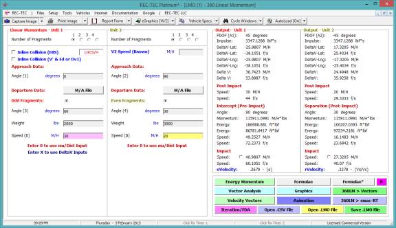
Figure 235 answers all of the questions.

Figure 236 displays the Graphics screen visually demonstrating that the centers of mass did not cross.

Figure 236

Figure 237

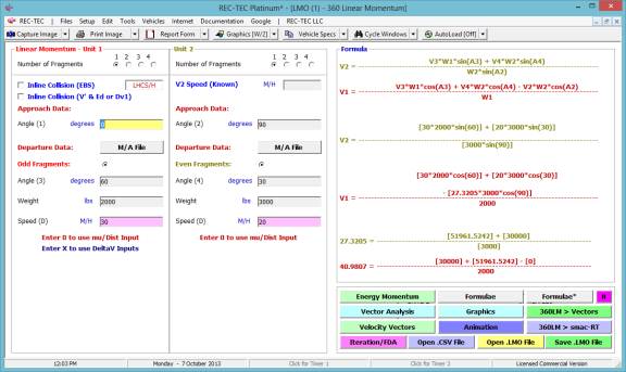
Figure 237 shows the formulae used in the computations.

Figure 238 shows the Vector Sum Analysis.

Figure 238

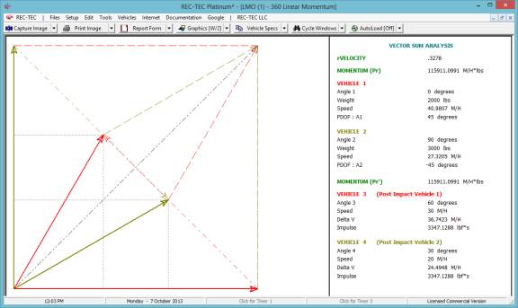
Figure 239

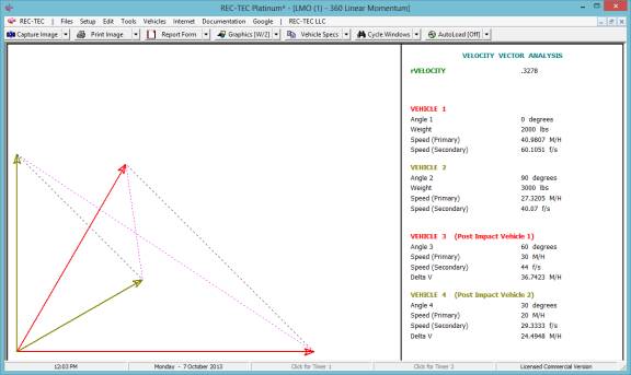
Figure 239 shows the Velocity Vectors and the resultant Closure and Separation vectors.

Figure 240 shows the Animation menu.

Figure 240

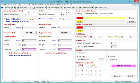
Figure 241

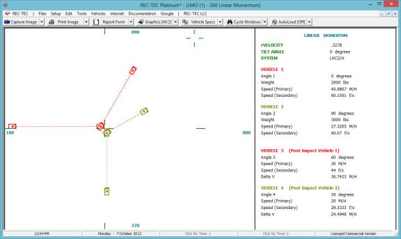
Figure 241 shows the animation with the vehicles colliding right-front to left-front.

Figure 242 shows the Graphics screen (See Figure 236) with the addition of the Plane of Impact for computing the Restitution (e) value for the collision.

Figure 242

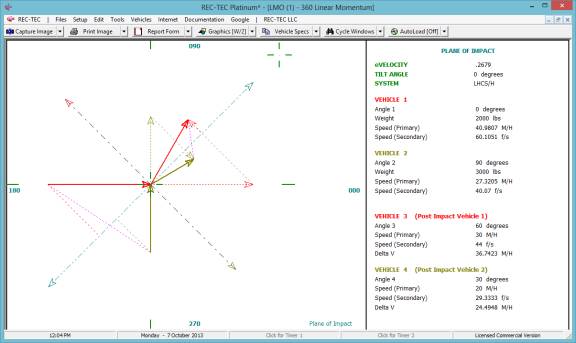
Before looking at Energy Momentum, we will look at Iteration and Finite Difference Analysis using the basic data out of Example 1.

Figure 243

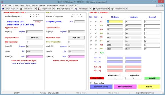
Figure 243 displays the Iteration/Finite Difference Analysis menu with ranges and intervals in place for the variables. The dV1 and dV2 blocks are left blank. The ranges would be used to show when values generated during iteration are outside of the specified ranges, showing those values in bold font.

Figure 244 shows a single variable table based on the value for angle 1 (A1).

Figure 244

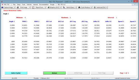
Figure 245

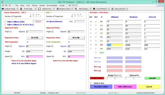
Figure 245 shows a two-variable iteration selection. Three pages will be generated for angle2 (A2) with each page showing a different weight for Vehicle1 (W1).

Figure 246 shows the A2 iteration for W1 @ 1750#.

Figure 246

Figure 247

Figure 247 shows the A2 iteration for W1 @ 2000#.

Figure 248 shows the A2 iteration for W1 @ 2250#.

Figure 248

Figure 249

Figure 249 shows the Finite Difference Analysis menu with the ranges for A1 removed. Leaving A1 has the effect of double dipping on the remaining angles as A1 does nothing more than shift the other three angles.

Figure 250 shows the Finite Difference Analysis.

Figure 250

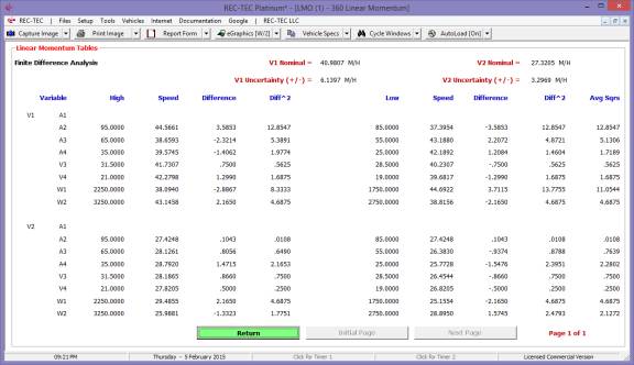
Figure 251

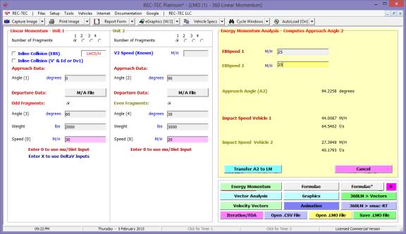
Figure 251 displays the Energy Momentum screen with the EBS values entered and the resultant computation for Angle 2 (A2) of 94.2258 degrees.

Figure 252 shows the A2 value transferred to Linear Momentum and the resultant solution.

Figure 252

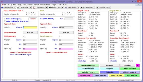
Figure 253

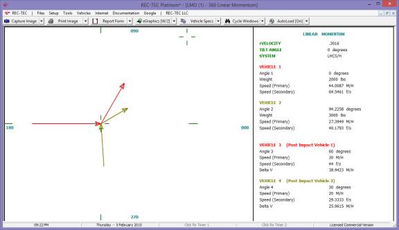
Figure 253 displays the Graphics for the changed Angle 2 (A2).

Figure 254 displays the Vector Sum Analysis for the changed Angle 2 (A2).

Figure 254

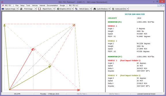
Example 2: Using the current data from Example 1 (with new A2 value of 94.2258 degrees), use Motion Analysis file Problem 19 as the post impact data for Vehicle 1. Enter zero (0) for the post impact speed of vehicle 2. Enter a 0.75 Mu, 100% braking, no grade, and a distance of 50 feet for Vehicle 2.

What are the impact speeds for both vehicles?

Figure 255

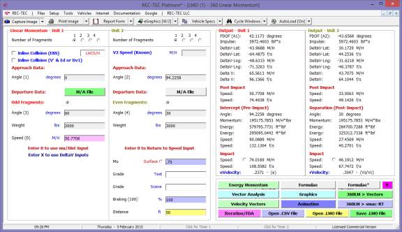
Figure 256 shows the Animation menu for Figure 257.

Figure 256

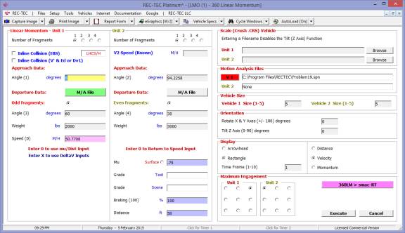
Figure 257

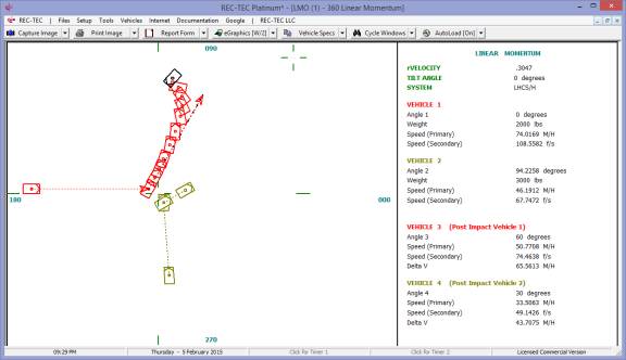
Figure 258 is the Vector Sum Analysis.

Figure 258

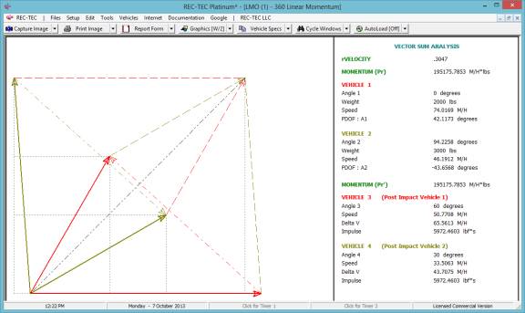
The impact speed for Vehicle 1 is 74.0169 M/H.

The impact speed for Vehicle 2 is 46.1912 M/H.

Note: To remove a Motion Analysis file Click on the M/A File button and then click on Cancel at either the warning message or the Dialog box.

Example 3: Open the .LMO file Frag8.LMO.

Figure 259

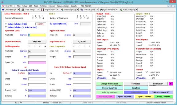
Figure 260 displays the graphics for all eight fragments and shows the angles, weights and speeds of each fragment.

Figure 260

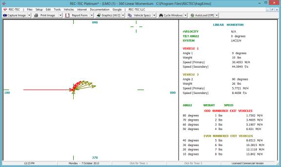
Figure 261

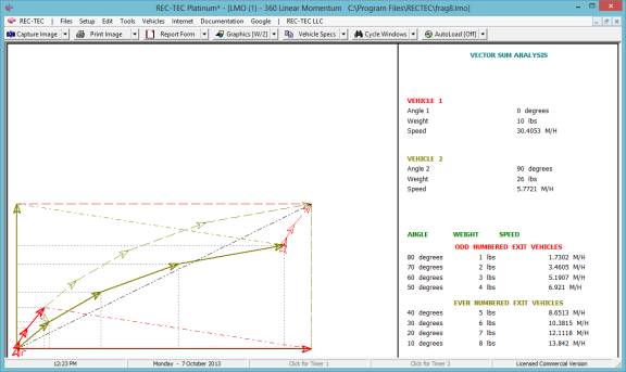
Figure 261 is the Vector Sum Analysis showing all eight fragments.

Figure 262 shows the first two fragments. Clicking on the Odd/Even fragment radio buttons will display the data for the specified fragments.

Figure 262

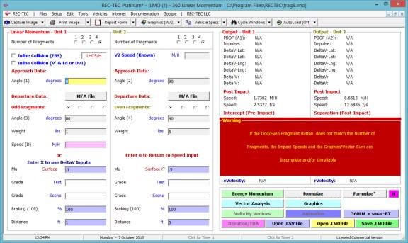
Example 4: Rear End Collision - Vehicle 1 (2500#) has a post –impact speed (V3) of 30. Vehicle 2 (2750#) has a post –impact speed (V4) of 30. V2 is stopped before collision. There is no EBS data available.

What is the impact speed of V1 and V2?

Figure 263

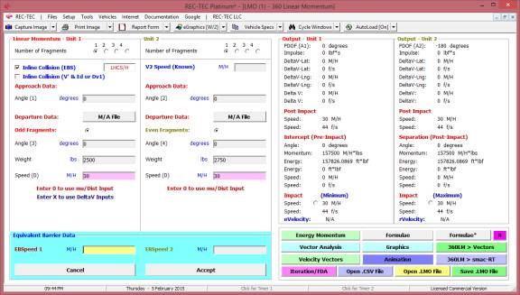
Figure 264

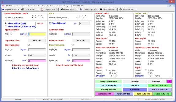
V1 speed = 63 M/H

V2 speed = 0 M/H

Figure 265

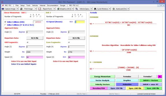
Figure 265 shows Formula used in the computation.

Figure 266 shows the Graphics.

Figure 266

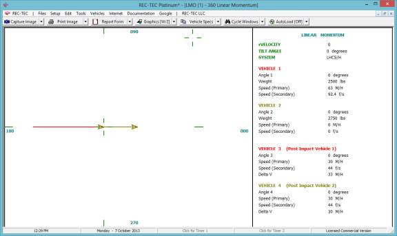
V1 speed = 63 M/H V2 speed = 0 M/H

Example 5: Vehicle 1 (2500#) has a post –impact speed (V3) of 30. Vehicle 2 (2750#) has a post –impact speed (V4) of 30. Vehicle 2 is moving at 20 M/H when it is rear-ended by Vehicle 1. No EBS Data is available. What is the impact speed of V1 and V2?

Figure 267

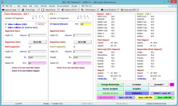
Figure 268

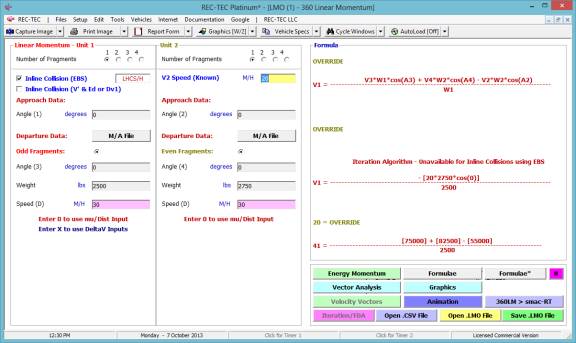
V1 speed = 41 M/H V2 speed = 20 M/H

Example 6: Vehicle 1 (2500#) has a post –impact speed (V3) of 30. Vehicle 2 (2750#) has a post –impact speed (V4) of 30. Vehicle 2 is moving at an unknown speed when it is rear-ended by Vehicle 1. The EBS for Vehicle 1 is 15 M/H and the EBS for Vehicle 2 is 17.5 M/H.

Figure 269

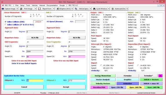
Figure 270

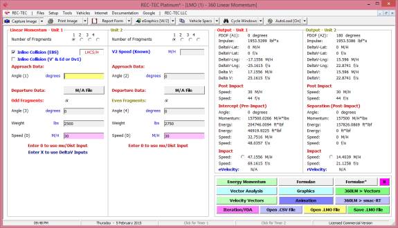
V1 speed = 47.1556 M/H

V2 speed = 14.4039 M/H

Example 6A: Vehicle 1 (5000#) is involved in a head-on collision with Vehicle 2 (4000#). CDR indicates a DeltaV of 29.54 for Vehicle 1. Scene evidence indicates the vehicles stuck together and that the post-impact speed was 22.68 M/H.

Figure 270A

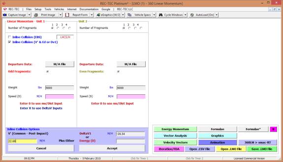
DV1 is entered as a negative value indicating a Head-on collision.

Figure 270B

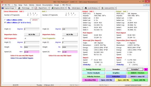
The program sets Angle 2 = 180 degrees based on the negative DV1 entry.

Figure 270C

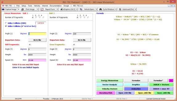
Formulae* brings up the Display in Figure 270C

Example 6B: Same as Example 6A except we will use a Energy from Damage value from CRUSH (Crash3) of 375,000 ft*lbf.

Figure 270D

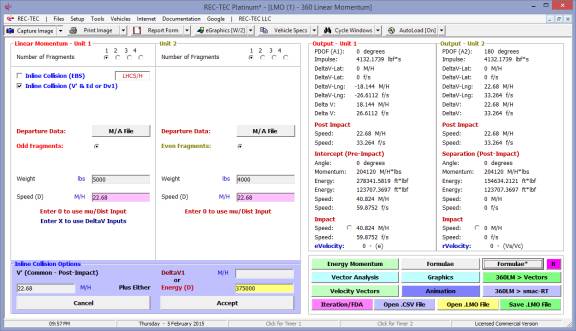
Figure 270E

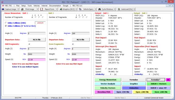
Figure 270F

The Head-on Collision (A2 = 180) results from the negative value computed for V2.

Example 6C: Same as Example 6A except we will use a Energy from Damage value from CRUSH (Crash3) of 75,000 ft*lbf. This results in a positive value for V2 indicating a Rear-end collision.

Figure 270G

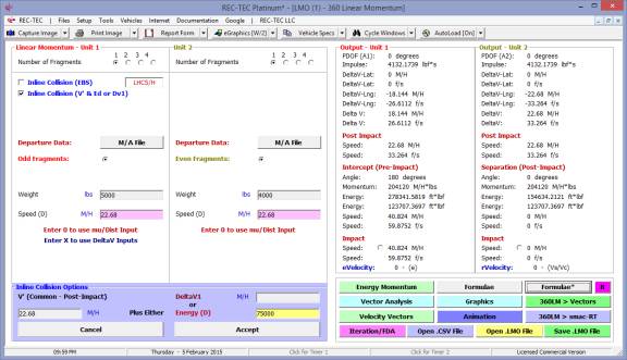
Figure 270H

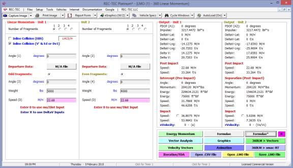
Figure 270I

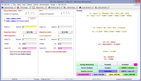
Example 7: Two vehicles skid over several different surfaces before colliding with each other. After impact, one of the vehicles (#1) skids 32 feet with a drag factor of 0.63 and runs off the roadway falling into a field. It will be assumed that the vault angle was 0 degrees; that the center of mass landed 8 feet below its takeoff height, and that landing was 43 feet downrange from the point of take off. Vehicle (#2) skids 47 feet on a .7 surface into a secondary collision with another object. Both skids assume (1) that the grade is level (0) and, (2) that all wheels were locked (100 % braking). Our objective is to determine the speed of the vehicles at the start of the pre-impact skids.

Figure 271

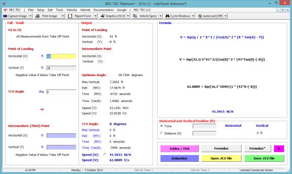
Figure 272

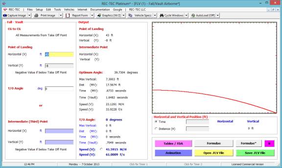
Figure 273

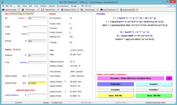
What is the post-impact speed for Vehicle #1?

Vehicle # 2 skids 47 feet on a .7 surface into a second collision. There are several ways to determine the impact speed for the second collision, including CRUSH, energy, and linear momentum. For this problem, we are going to assign an impact speed of 12.5 M/H for the second collision.

Figure 274

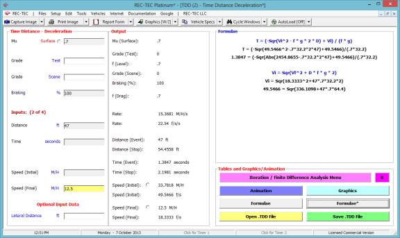
What is the post-impact speed for vehicle #2?

ASSUMED FOR PROBLEM:

Vehicle #1: 2750 pounds

Pre-impact A1 = 350 degrees (LHCS/H)

Post-impact A3 = 60 degrees (LHCS/H)

Vehicle #2: 2500 pounds

Pre-impact A2 = 100 degrees (LHCS/H)

Post-impact A4 = 30 degrees (LHCS/H)

REC-TEC will operate using both the right and left hand coordinate systems. In this example the Left-hand system (LHCS) will be used. REC-TEC can use either heading angles or radial angles for the approach angles of the vehicle. Heading angle uses the angle in which the vehicle is headed. (In the RHCS, if the vehicle were traveling from left to right, the heading angle would be 90 degrees. Radial angle uses the angular position of the vehicle before impact. In the RHCS if the vehicle were traveling from left to right, then the radial angle is 270 degrees.)

Figure 275

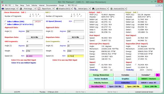
Figure 275B shows all four screens in this problem simultaneously.

Figure 275B

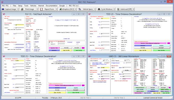
Did the centers of mass of the two vehicles cross?

What is their closure angle?

What is their separation angle?

What is the impact speed of vehicle #1?

What is the impact speed of vehicle #2?

What is the PDOF of vehicle #1?

What is the PDOF of vehicle #2?

What is the DeltaV of vehicle #1?

What is the DeltaV of vehicle #2?

Run a Vector Sum Analysis. Does it work?

Figure 276

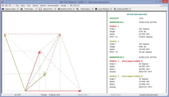
Rerun the problem and override the computed answer for Vehicle #2 using 60 M/H. Run a Vector Sum Analysis. Does it work?

Figure 277 

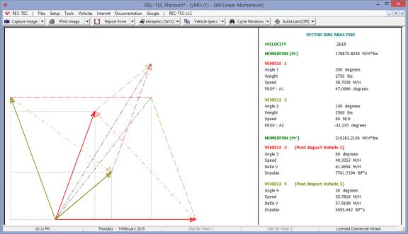
The resultant vectors in Figure 277 should overlap and meet at a common point as in Figure 276.

Module 25: Momentum – 360 LM Omni - PDOF Lite (V1 and/or V2)

(Table of Contents)

Overview: This module computes the Impact Speed, DeltaV and PDOF data for angular collisions. As of September 2017 it replaces Vector Momentum (Module 28)

This module was upgraded in 2017. The new images are shown.

At the REC-TEC pull down menu, select Momentum > 360 LM Omni-PDOF Lite (V1 and/or V2) and the 360 LM Omni-PDOF Lite screen appears (Figure 278).

Figure 278

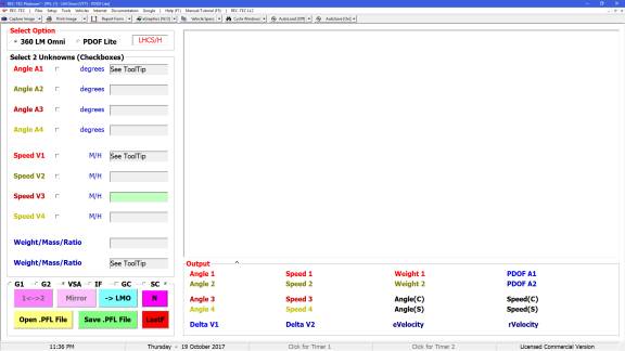
Required Input Data

In PDOF Mode (Either Vehicle):

· Approach Angle

· Departure Angle

· Approach Speed

· Departure Speed

In 360 Momentum Mode (requires data on both vehicles)

· Approach Angles

· Departure Angles

· Approach Speeds

· Departure Speeds

· Weights

Weights of the vehicles are required. The other 8 variables may contain 2 unknowns. User may select unknowns using the checkmarks shown on the interface.

Example 1: Vehicle 1 (3700#) traveling due east collides with Vehicle 2 (2500#) traveling due southwest (235 degrees). V1 exits at 335 degrees at speed of 15 M/H, while V2 exits at 305 degrees at 25 M/H.

What is their closure angle?

What is their separation angle?

What is the impact speed of both vehicles?

What is the PDOF of both vehicles?

What is the DeltaV of both vehicles?

Figure 279

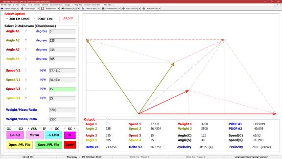
The 360-degree formulae used in the above computations solve for V1 and V2 independently. They may be used independently to solve for a particular unknown in question. They may be only be used with the Left Hand Coordinate System with V1 on a heading of 0 degrees. This shows the Vector Sum Analysis diagram by default.

Figure 280A

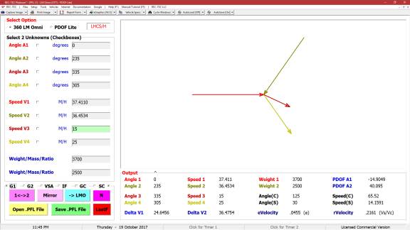
Figure 280A shows the G1 diagram.

Figure 280B

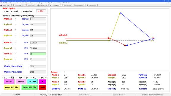
Figure 280C shows the formulae after Speed V1 and Speed V2 were chosen as Unknowns and the IF radio button is selected.

Figure 280C

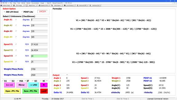
Figure 280D

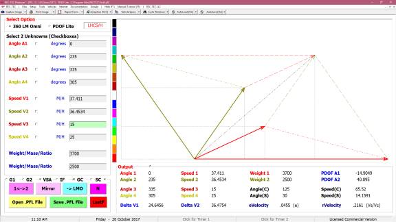
Figure 280D shows the problem using the Vector Sum Analysis graphic. It also shows the LM Omni color palate for drawing on all graphics screens in REC-TEC.

Figure 280E

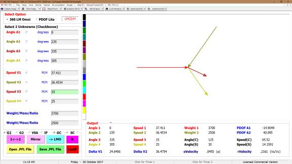
Figure 280E shows the problem using the G1 graphic. It also shows the REC-TEC color palate for drawing on all graphics screens in RECTEC.

Figure 280F

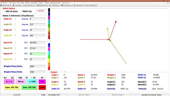
The above Graphic shows the diagram after selecting the [1 < - > 2] button, which places Vehicle 2 at 0 degrees on the horizontal axis and moves Vehicle 1 to a relative position on the screen. Note: REC-TEC will show the VSA graphic immediately after switching to check that the switch worked correctly.

Figure 280G

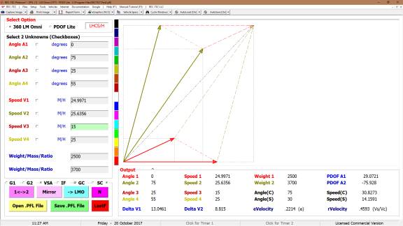
Figure 280G shows problem file Test2.pfl. This problem will be used to demonstrate Vector Triangulation Technology (VTT), a new feature introduced in 360 LM Omni. While other software will allow the user to solve for the linear momentum approach and departure speeds using the Colorado School of Mines formulae variants introduced in REC-TEC roughly 20 years ago, VTT now allows both the angles and the speeds to be treated as unknowns.

Figure 280H

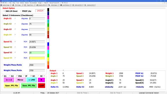
Note that Angle A3 (departure angle for Vehicle 1), and Speed V4 (departure speed for Vehicle 2), are both blank, with no solution shown. As soon as the checkboxes for both of these variables are marked, the VTT solution will be shown.

Figure 280I

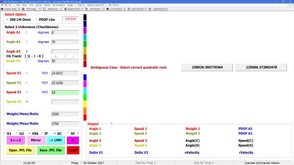
Selecting an answer will show the solution for that choice. The second choice will be selected,

Figure 280J

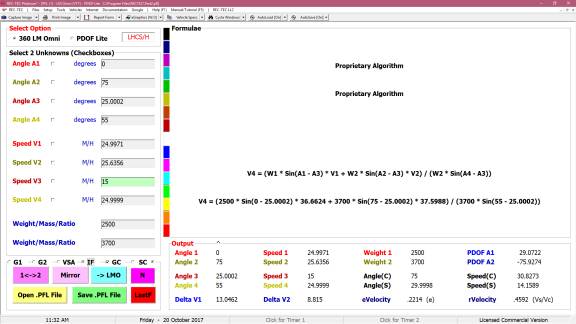
Figure 280J shows the Formulae for V4. Angle A3, and all of the angle computations are computed using the proprietary algorithm (VTT) developed by REC-TEC.

Figure 280K

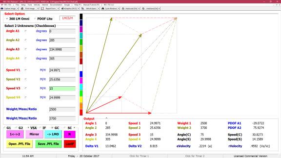
Figure 280K displays the VSA Graphic image Mirrored on the other side of the Horizontal axis.

Figure 280L

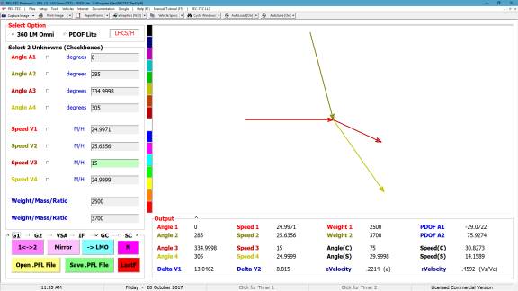
Figure 280L displays the G1 Graphic image Mirrored on the other side of the Horizontal axis.

Solving for Impact and Post-Impact Speeds in 360 LM Omni

REC-TEC uses a method of solving for the impact and post-impact speeds in a collision using the Law of Sines, the Law of Cosines, and Newton’s Third Law of Motion. This methodology dispenses with the necessity of doing a Trajectory Analysis on both vehicles post-impact and then marrying these analyses with the Damage Analysis. This methodology also has the added benefit of serving as a crosscheck on the trajectory analysis.

This method requires the following inputs from CRUSHV, 360 LM, or User:

Longitudinal DeltaV (X) - (Computed in Crush & 360 LM)

PDOF1 (Degrees) – (Computed in 360 LM)

Angle 1 (Degrees) – Always Zero (0)

Angle 2 (Degrees) – Input by User

Angle 3 (Degrees) – Input by User

Angle 4 (Degrees) – Input by User

Weight (1) – Input by User

Weight (2) – Input by User

With Crash Data Retrieval (CDR) downloads becoming increasingly available, this new methodology offers a valuable alternative to the V3 and V4 requirement, one not always as reliable or accurate as desired. It also offers a convenient crosscheck when V3 and V4 are available. It does require the Approach and Departure angles, but those are also required for a traditional Trajectory Analysis. CRUSHV & 360 LM Omni modules use the Left Hand Coordinate System – Heading angles and use Zero (0) for Angle 1.

Formulae:

DV1 = DV1X / Cos(PDOF1 + Abs(SlipAngle))

DV2 = DV1 * (W1 / W2)

AngleC = 180 - (A3 + PDOF1)

AngleA = A2 - A4

PDOF2 = 180 - (PDOF1 + A2)

AngleB = 180 - (PDOF2 + AngleA)

V1 = DV1 * Sin(AngleC) / Sin(A3)

V3 = DV1 * Sin(PDOF1) / Sin(A3)

V2 = DV2 * Sin(AngleB) / Sin(AngleA)

V4 = DV2 * Sin((180 - (AngleB + AngleA)) / Sin(AngleA)

Hints on getting the most out of this “new’ Module:

· This Module must be run using the Left Hand Coordinate System / Heading Angles with V1 on a heading of 0 degrees.

• CrushV can send data to 360 LM Omni, which can send the data to 360 LM for additional processing and analization.

• Computations for unknowns requires 2 unknowns be selected. If you only need one, pair it with Angle 1, as Angle 1 must be Zero (0).

• If selecting Angle 3 and Angle 4 as the Unknowns, the program cannot determine if the CGs of the Vehicles cross. The program will offer the user the option of crossing the CGs, having the CGs follow the same Track, or not having them cross. To have the vehicles stick together, Speeds 3 & 4 must be Identical.

• REC-TEC grants access to all 28 combinations of Angles and Speeds as Unknowns in this module. It is sometimes necessary for the VTT algorithm to make Square Root computations. A negative root is never permitted, but occasionally there will be 2 positive roots. Both roots will be displayed and the user must choose the correct root. If final answers are desired for both positive roots, reselect the unknowns and choose the alternate root.

• On some computations, the VTT algorithm may need to know if the angular difference between Angle 1 and Angle 2 (Approach angles) is greater than or less than 90 degrees (Difference < 90 or > 90).

• Inputs, when brought into the computations by loading a file, are, by default, truncated at the 4^th decimal position. This can create a small change at the 4^th and sometimes even in the 3^rd decimal position. It is caused by the truncation of the inputs.

• When a Variable is selected as an unknown using the Checkbox, the information for that Variable is cleared as if it had never been entered. The program removes it from the computations, treating it as a Zero (0).

• If any Variable is manually changed by the user, then the Primary Solutions (V1 and V2), or (V3 and V4), must be selected as unknowns and solved for by the program. The decision to not automatically resolve the problem was made because V1 and V2 may not be the Variables that are the unknowns. This decision is left to the user, but must not be ignored and will be displayed in the VSA graphic displayed by default. The VSA graphic demonstrates whether or not the “unknowns” required for the problem must be resolved.

• Next year at the earliest, there is a small chance that we may release a workbook describing in detail how the VTT algorithm reaches its solutions. That information is not required as 360 LM can take the information generated and show that it is accurate. For now that information is proprietary.

Module 26: Momentum – Angular Momentum

(Table of Contents)

Overview: This module computes the speed of a striking vehicle using pre- and post-impact data in conjunction with inertial and rotational information.

At the REC-TEC pull down menu, select Momentum > Angular Momentum and the Angular Momentum screen appears (Figure 281).

Figure 281

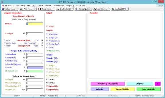
Required Input Data

Mass Moment of Inertia

· Inertia - Enter the Yaw Moment of Inertia

Or

· V1 Length – Length of Vehicle 1

· V1 Center to CG – Distance from Center of Vehicle to CG of Vehicle

· V1 Width – Width of Vehicle 1

Plus

· V1 Weight – Weight of Vehicle 1

Rotation Point (Set appropriate Radio buttons)

· CCW – Counter-Clockwise Rotation

· CW – Clockwise Rotation

· CG (Hi Spd) – Rotation about CG (Usually a High Speed Rotation)

· Axle (Low Spd) – Rotation about Center of Axle (Usually a Low Speed Rotation)

· Damage Point – Select Front or Rear Location Point of Damage

Torque & Rotational Velocity

· V1 Wheelbase – Wheelbase of Vehicle 1

· V1 Weight (A) – Weight on V1 Axle closest to Centroid of Damage

· V1 Friction (mu) – Surface Friction for Tires on Axle closest to Centroid of Damage / All Tires

· V1 Rangle (Degrees) – Rotation Angle of Vehicle in degrees

· V1 Dcom – (Low Speed Rotation Only) – Distance from the Center of Mass of the vehicle to the Axle farthest from the Centroid of Damage.

· V1 Moment Arm

1. Low Speed Rotation – a line from (and perpendicular to) the PDOF to the center of farthest Axle from Centroid of Damage (Center of Rotation)

2. High Speed Rotation –a line from (and perpendicular to) the PDOF to the Center of Mass (Center of Rotation)

Delta V & Impact Speed

· V2 Weight – Weight of V2

· V2 AAngle (degrees) – Approach Angle of Vehicle 2

· V2 DAngle (degrees) – Departure Angle of Vehicle 4

· V2 Speed (V4) – Departure Speed of Vehicle 2

Help File – The paper “Motorcycle Speed Estimates Using Conservation of Linear and Rotational Momentum” by Bruce F. McNally, Northeast Collision Analysis, Inc. and Wade Bartlett, PE, Mechanical Forensics Engineering Services, LLP. This paper was presented at the 20th Annual Special Problems in Traffic Crash Reconstruction at the Institute of Police Technology and Management, University of North Florida, Jacksonville, Florida, April 15-19, 2002. It is an exceptional discussion of Angular Momentum as applied to accident reconstruction. The paper is used with the express written permission of the authors. REC-TEC wishes to express our thanks to them for job well done and for their gracious permission to use their paper.

The following examples are taken from the paper “Motorcycle Speed Estimates Using Conservation of Linear and Rotational Momentum.”

Figure 282

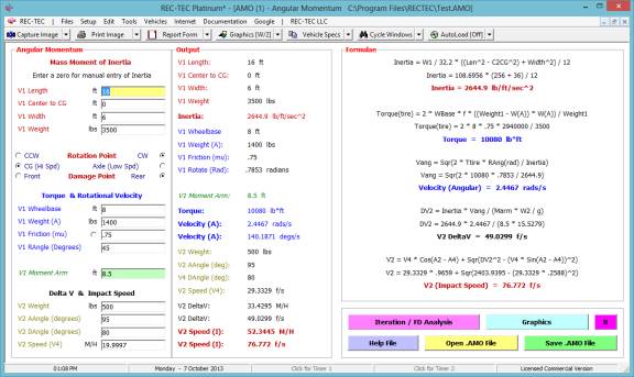
Figure 283 shows the Graphics for the first example shown in Figure 282.

Figure 283

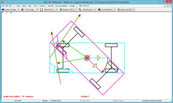
Figure 284

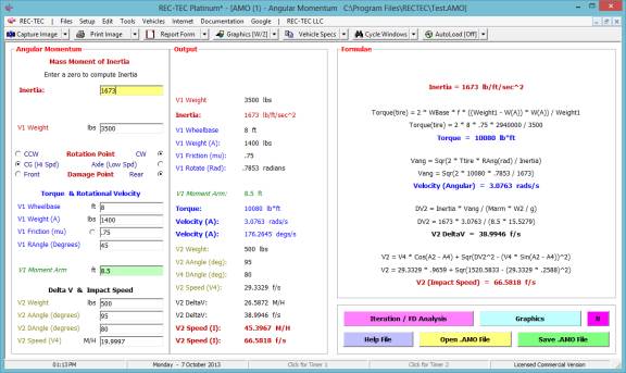
Figure 285 shows the Graphics for the second example shown in Figure 284.

Figure 285

Figure 286

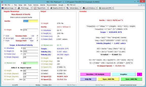
Figure 287 shows the Graphics for the second example shown in Figure 286.

Figure 287

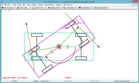
Figure 288 shows the Iteration/Finite Difference Analysis menu with a range of values for the problem shown in Figure 286.

Figure 288

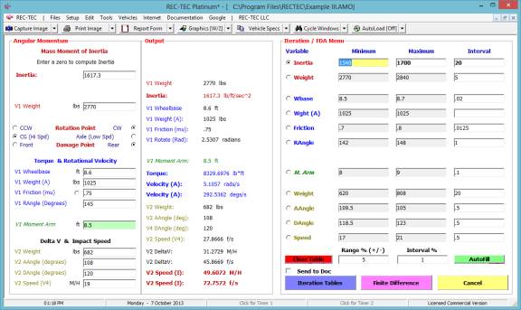
Figure 289 shows the Iteration table for the variable and values selected in Figure 288.

Figure 289

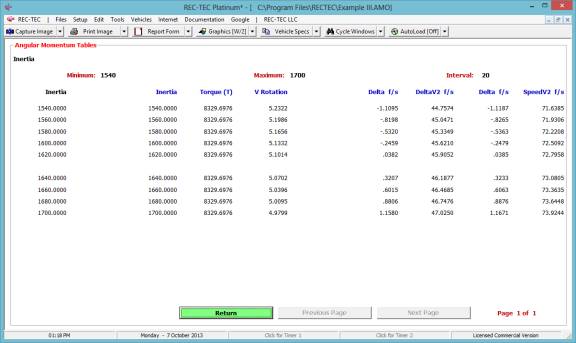
Figure 290 shows the Finite Difference Analysis for the range of values specified in Figure 288.

Figure 290

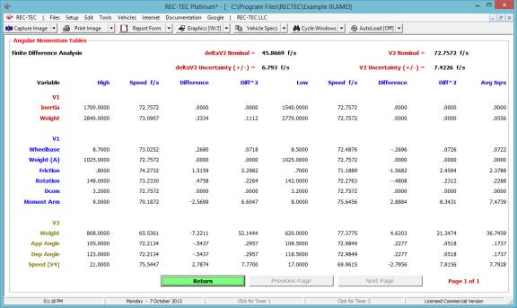
Figure 291 uses the same information as seen in Figure 286 with the exception of the Rotation Point, which in this case is changed to Axle (Low Spd). The resulting Graphics are shown in Figure 292.

Figure 291

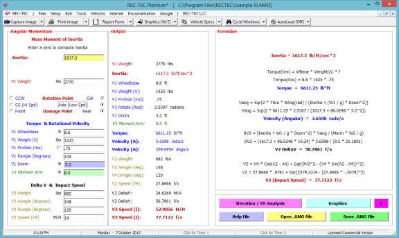
Figure 292

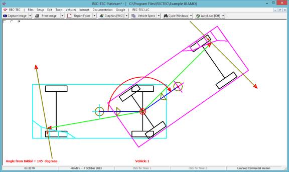
The graphics in this section are somewhat generic except for the positioning of the vehicles. This enables the module to show what is occurring in the rotation without going into detail about the dimensional characteristics of the vehicle, the damage characteristics including the PDOF for each vehicle.

Module 27: Momentum – Low Speed Collisions

(Table of Contents)

Overview: This module computes the Closure Speed and DeltaV data in Low Speed Collisions.

At the REC-TEC pull down menu, select Momentum > Low Speed Collisions and the Low Speed Collisions screen appears (Figure 293).

Figure 293

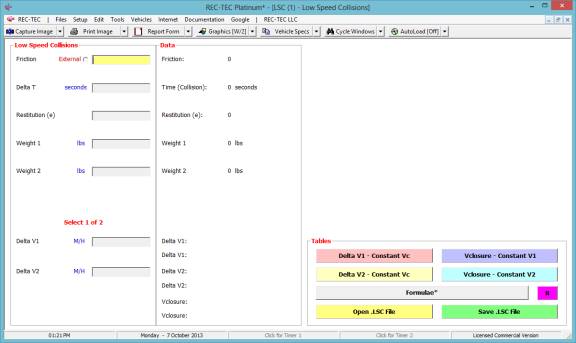
Required Input Data

· Friction (External) – Sum of the External Friction Forces

· DeltaT – Time of the Collision

· Restitution (e) – Restitution value for the Collision

· Weight 1 – Weight of Vehicle 1

· Weight 2 – Weight of Vehicle 2

· Delta V1 – Change of Velocity for Vehicle 1

Or

· Delta V2 – Change of Velocity for Vehicle 2

This module requires a unique and sometimes difficult to obtain set of variables. The external friction will generally be the surface friction, but it can include the frictional forces between the vehicles. The DeltaT will generally be in the neighborhood of 100 milliseconds (.1). This value can sometimes be obtained using a SMAC program. DeltaV and Restitution can be computed using Linear Momentum. The module will build a table based on a wide range of variables. The screens below will show different options for a given set of input variables.

Example 1: Friction = 0.3, DeltaT = 0.1, Restitution = 0.24, W1 = 3617#, W2 = 2149#, and DeltaV1 = 2.0454.

Figure 294

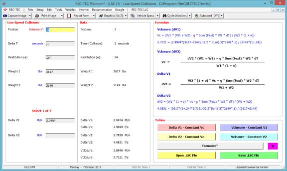
Figure 295 shows the table for Delta V1 – Constant Vc.

Figure 295

Figure 296 shows the table for Delta V2 – Constant Vc.

Figure 296

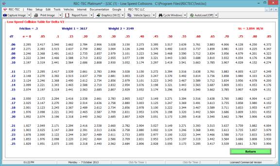
Figure 297 shows the table for Vclosure – Constant V1.

Figure 297

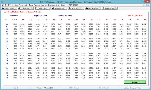
Figure 298 shows the table for Vclosure – Constant V2.

Figure 298

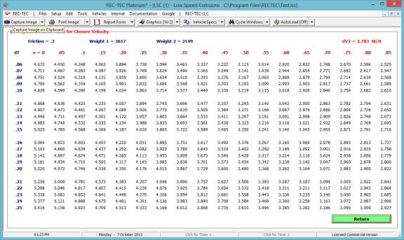
Module 28: Momentum – Vector Momentum Analysis

(Table of Contents)

(Replaced by Module 25)

Module 29: Energy - Damage Analysis > Crash3 (Crush5 - DeltaV from Damage)

(Table of Contents)

Overview: This module uses enhanced Crash3 Damage Analysis algorithms to compute collision data including Delta V (change of velocity) for the collision. If angular information is supplied, the pre and post impact speeds are also computed as well as the closing velocity (Vc).

Note: In October 2015 the Closing Velocity (Vc) was found to be so unreliable that it is no longer displayed unless COLM angles are furnished integrating Vector Analysis and Crush5 making the Vc computation very accurate.

At the REC-TEC pull down menu, select Energy - Damage Analysis > Crash3 (Crush5 - DeltaV from Damage and the Crush5 screen appears (Figure 306).

Figure 306

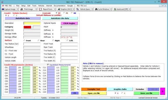
Required Input Data

This module contains the following data entry blocks:

Crush5

Centroid:

• RT – REC-TEC Equations for Centroid

· PE – Parkka Equations for Centroid

· ME – Mitchell Equations for Centroid

Vehicle:

· Vehicle 1

· Vehicle 2 (If second vehicle)

Description – Vehicle (N) Description (Optional)

Category

· Default – Sets defaults for Entered Vehicle Category

· Textbox – Entry of Category for Vehicle (Zero for no Category)

· Weight – Weight of Vehicle

· Damage Width – Width of Damage (L)

· Damage Offset – CG is reference point. If damage is forward or right, use a positive value; if rearward or left, use a negative value.

· PDOF – 0 to +/- 180 degrees 0 = Front, 180 = Rear, -90 = Left, +90 = Right

· Stiffness A – Stiffness Coefficient A

· Stiffness B – Stiffness Coefficient B

· Stiffness G - Computed be program

Surface (Damage Location – Select by Radio button)

· Front

· Rear

· Right

· Left

· Yaw Radius of Gyration – Leave blank to have program compute

· Wheelbase – Front axle to Rear axle

· CG – Front Axle – Distance from CG to Front Axle

· CG – Front – Distance from CG to Front

· Vehicle Length – Length of Vehicle

· Vehicle Width – Width of Vehicle

Optional Data (for Scale Diagram in Graphics only - does not enter computations)

· Front Track

· Rear Track

· Tire Radius (F)

· Tire Radius (R)

· Tire Width (F)

· Tire Width (R)

Crush Measurements (2 minimum / 20 maximum)

· C01 to C20 - Use as required

· L01 to L20 – Cumulative Distance from L01. L01 is always Zero (0).

· % (19) – Weight for Segment as percent (1 to 100) defined by adjacent “C” measurements

Non Linear Crush5 Functions (Check to Enable)

Percent of “C” Measurement

• Zone (1 to 3) – Length of “C” enables defining three separate Zones
• Percent – Weight for Zone as percent (1 to 100) defined by length of “C” measurements
  or
• Inches of “C” Measurement

· Zone (1 to 3) – Length of “C” enables defining three separate Zones

Weight for Zone

· Percent – Weight for Zone as percent (1 to 100) defined by length of “C” measurements

Test Collision Data (Used to compute A, B & G Stiffness Coefficients)

· Crush Energy Equivalent Speed – Exemplar Vehicle in Test Crash (See Module 31)

· Maximum CEES without Permanent Damage (B₀)

· Average Crush – Enter 0 (Zero) to Compute

· Number of “C” Measurements

· Length of (Each) “C” Measurement

· Test Vehicle Weight – Exemplar Vehicle in Test Crash

· Test Vehicle Damage Width – Exemplar Vehicle in Test Crash

Example 1: This example will explain the features available on the screen while filling in the data.

Collision Force Error – Two red Command Buttons (Figure 308) with the Collision Force for Vehicle 1 and Vehicle 2 appear in the Crush5 Analysis Output frame if there is an imbalance of the Collision Forces between the vehicles. Click on the Collision Force to be changed to engage a frame that shows the information required to balance the Collision Forces of the vehicles.

Figure 307

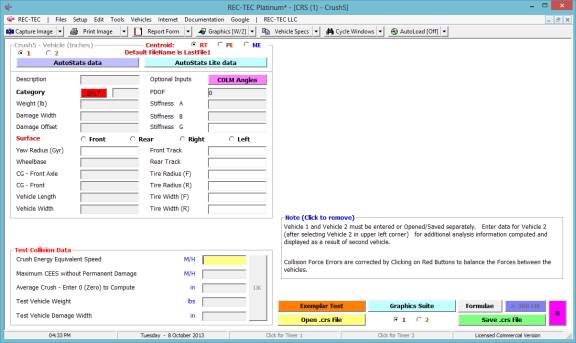
Figure 307 displays the Test Collision Data frame resulting from clicking on the Exemplar Test button. This frame will assist in computing the A and B stiffness values for the vehicle as shown in Figure 308.

Figure 308

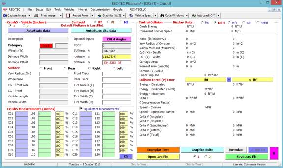
The AutoStats button will be used to call up the Vehicle Exchange Files produced by the commercial Autostats program. Later the Autostats Lite button will be used for Vehicle 2.

Figure 309

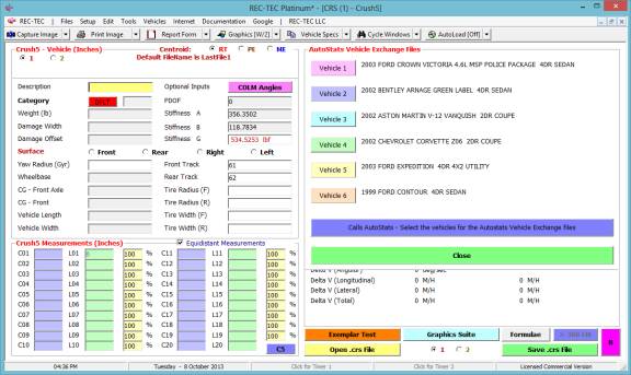
Selecting Vehicle 3 from the Vehicle Exchange Files results in the transfer of data shown in Figure 310.

Figure 310

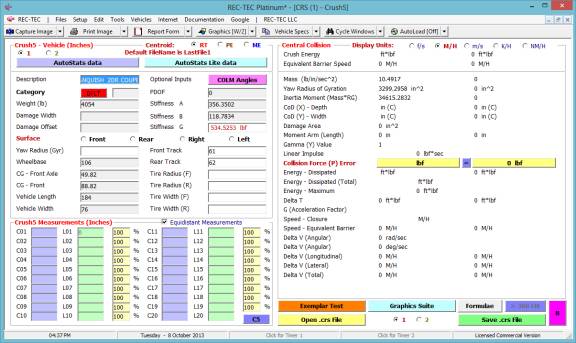
Damage Width, Damage Offset, Damage Surface and tire information is added in Figure 311. The PDOF will be left at zero for this frontal collision.

Figure 311

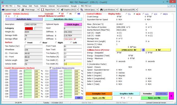
Damage is the same as it was on the Exemplar vehicle test with 15 inches of crush across the entire front of the vehicle.

Figure 312

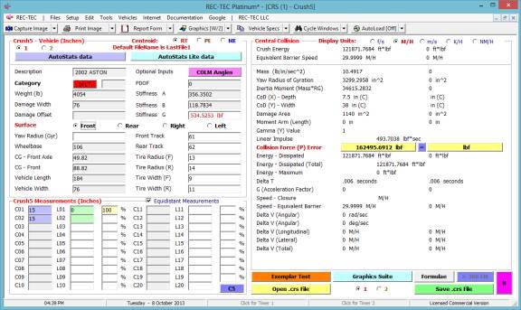
Based on this information the module generates an EBS of 29.9999 M/H. Remember, REC-TEC computes to 21 places and truncates. This sure is close to 30 M/H entered for the speed of the Exemplar vehicle. Clicking on the Graphics Suite button will bring up Figure 313.

Figure 313

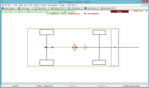
In Figure 313 there are four buttons allowing us to move up, down, right, and left. There is also a Reset button and a checkbox that will permit the adjustment of the CoD (Centroid of Damage). At the bottom of the graphics screen (Figure 313) a scale will make the vehicle bigger or smaller to fit the screen, or zoom in on a particular feature.

The screen also states that it is using REC-TEC equations. This is for the computation of the CoD. The module will allow use of three different sets of equations to compute the CoD. The selection is made at the upper left center of the screen (Figure 312) by Radio button. Please see the suggested reading materials at the end of this section for additional information concerning this selection. It is recommended that the user never change from the REC-TEC selection as the two others are dramatically flawed (See Proof of Concept below).

This is about as far as we can go using a single vehicle CRUSH program. REC-TEC offers the ability to use two vehicles in collision in the Damage Analysis component of the CRASH3 program.

Example 2: Vehicle 1 from Example 1 will now collide with the side of Vehicle 2, which is stopped in order to make some things a bit simpler. Notice there was no DeltaV computation in Example 1. We do not know what occurred post-impact. This situation will change with the addition of another vehicle. Click the Vehicle 2 radio button in the upper left of Figure 314 and we will get started.

Figure 314

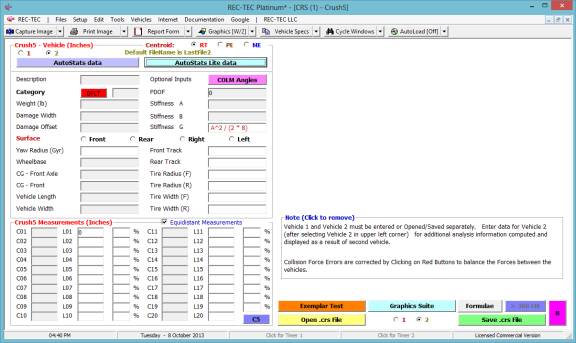
It looks like we are back to where we started, except now the module wants data on Vehicle 2, a Mazda MX-5 Miata, 2-door convertible. We have determined that this is a Category 1 vehicle. The default A and B values will be used. Enter a “1” for the Category and Click on “DFLT.”

Figure 315

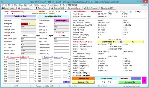
For specific data on our vehicle, click on the Autostats Lite button to find data on Vehicle 2, a Mazda MX-5 Miata, 2-door convertible (Figure 316).

Figure 316

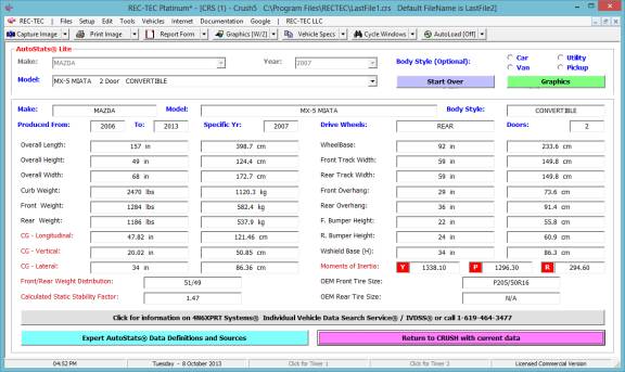
Click on the red “Return to CRUSH with current data” button and the data will be ready to transfer to Vehicle 2 as shown in Figure 317.

Figure 317

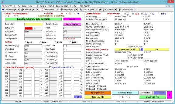
Clicking on the “Transfer Autostats Data” to Crush places the dimensional data as shown in Figure 318.

Figure 318

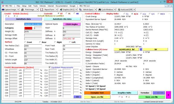
The damage is on the left side of the vehicle. The damage width is measured at 96 inches and is centered 10 inches forward of the center of gravity (cg) of the vehicle. The PDOF is – 90. Tire information has also been added.

Figure 319

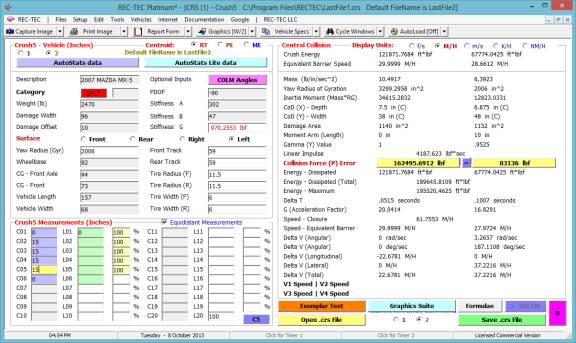
With the addition of the second vehicle, the module can now generate DeltaV information and a lot more. However, there is a collision force error. The stiffness values for Vehicle 1 were computed from an exemplar test and are more reliable that the approximated values for a generic Category 1 vehicle. Crush Measurement data has been added. As a precaution, remove the “1” from the Category textbox so that the vehicle data will be secured.

Click on the Yellow Collision Force button for Vehicle 2 to balance the force to that of Vehicle 1 that has a higher degree of confidence, bringing up Figure 320.

Figure 320

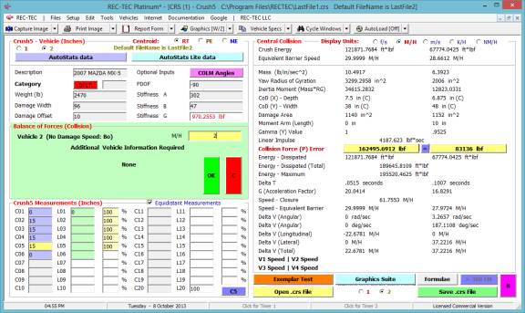
Enter a value of “2” for the no damage speed for the side of Vehicle 2 and click “OK.”

Figure 321

The data on Vehicle 1 is shown in Figure 321 along with the analysis for both vehicles. Note that the total DeltaV for Vehicle 1 is only 24.4025 M/H even though the EBS remains at 29.9999 M/H.

Figure 322

The data on Vehicle 2 is shown in Figure 322 along with the analysis for both vehicles. The Graphics will be shown in Figures 323 through 326. The total DeltaV for Vehicle 2 is 40.0518 M/H and the EBS is 34.4139 M/H.

Figure 323

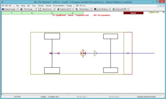
Figure 323 shows the scale graphics for Vehicle 1.

Figure 324

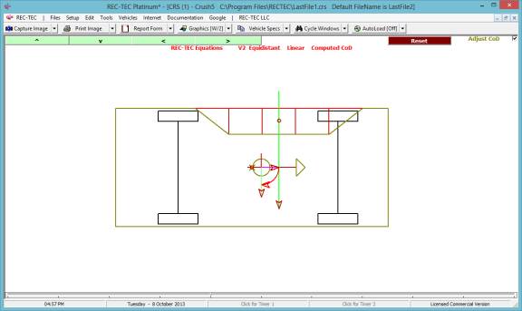
Figure 324 shows the scale graphics for Vehicle2.

Figure 325

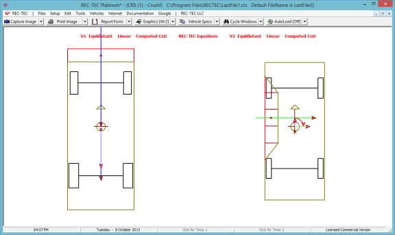
Figure 325 shows the scale graphics for Vehicle 1 and Vehicle 2 compared side-by-side.

Figure 326

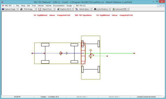
Figure 326 shows the scale graphics for Vehicle 1 and Vehicle 2 integrated into collision with the centroids of damage overlapped and the supplied PDOFs shown as equal and opposite.

Example 3: Open the vehicles used in the Digital Momentum (Module 23 - Figure 221 - Example 3) for analysis in CRUSH. The file “Car1.crs” was used for Vehicle 1. The file “CAR1A.CRS” was used for Vehicle 2. Figure 327 shows both files loaded into the CRUSH module.

Figure 327

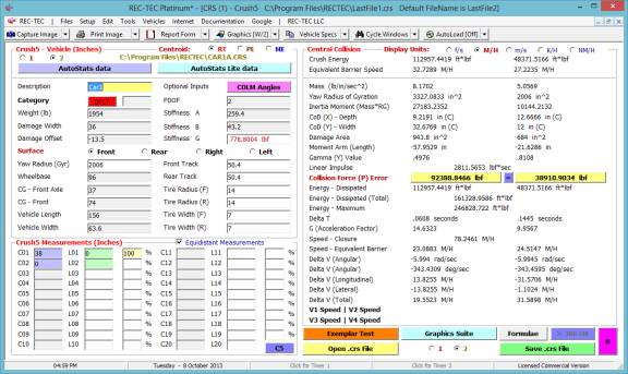
Figure 328 shows Vehicle 2 balanced to Vehicle 1. No damage speed = 5.

Figure 328

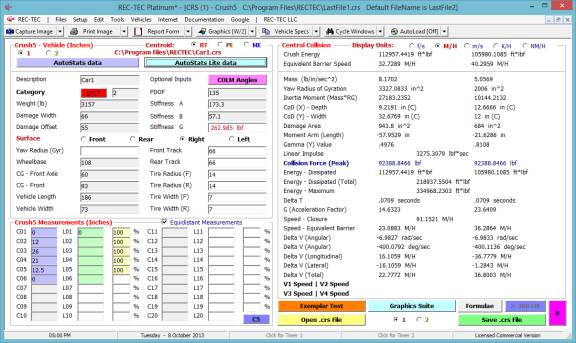
Figure 329

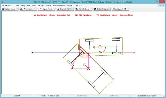
Figure 329 shows both of the vehicles integrated into collision as they were in Module 23.

Figure 330

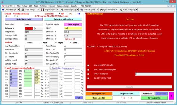
Figure 330 displays the Caution Message resulting from changing the PDOF angle of Vehicle 1 to 140 degrees and the options available. Figure 331 shows the results of using the computed multiplier.

Figure 331

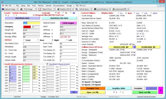
Figure 332

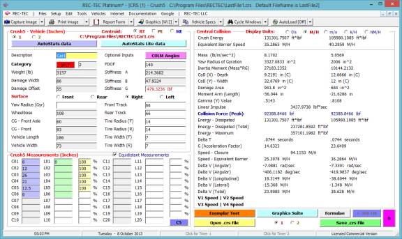
Figure 332 shows Vehicle 1 balanced to Vehicle 2.

Figure 333

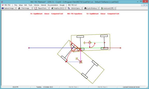
Figure 333 shows both of the vehicles integrated into collision using the revised data.

Solving for Impact and Post-Impact Speeds in CRUSH

(Table of Contents)

REC-TEC uses a method of solving for the impact and post-impact speeds in a collision using the Law of Sines, the Law of Cosines, and Newton’s Third Law of Motion. This methodology dispenses with the necessity of doing a Trajectory Analysis on both vehicles post-impact and then marrying these analyses with the Damage Analysis. This methodology also has the added benefit of serving as a cross check on the trajectory analysis.

This method requires the following inputs:

Longitudinal DeltaV (X) - (Supplied by CRUSH)

PDOF1 (Degrees) – User supplied in CRUSH

Angle 2 (Degrees) – Input by User

Angle 3 (Degrees) – Input by User

Angle 4 (Degrees) – Input by User

Weight (1) – User supplied in CRUSH

Weight (2) – User Supplied in CRUSH

With Crash Data Retrieval (CDR) downloads becoming increasingly available, this new methodology offers a valuable alternative to the V3 and V4 requirement, one not always as reliable or accurate as desired. It also offers a convenient cross check when V3 and V4 are available. It does require the Approach and Departure angles, but those are also required for a traditional Trajectory Analysis. The REC-TEC CRUSH module uses the Left Hand Coordinate System – Heading angles and uses Zero (0) for Angle 1.

Formulae:

DV1 = DV1X / Cos(PDOF1 + Abs(SlipAngle))

DV2 = DV1 * (W1 / W2)

AngleC = 180 - (A3 + PDOF1)

AngleA = A2 - A4

PDOF2 = 180 - (PDOF1 + A2)

AngleB = 180 - (PDOF2 + AngleA)

V1 = DV1 * Sin(AngleC) / Sin(A3)

V3 = DV1 * Sin(PDOF1) / Sin(A3)

V2 = DV2 * Sin(AngleB) / Sin(AngleA)

V4 = DV2 * Sin((180 - (AngleB + AngleA)) / Sin(AngleA)

Example 1

This example will use two identical vehicles except for the weights in a 90-degree collision and identical 45-degree PDOFs.

Figure 333-1

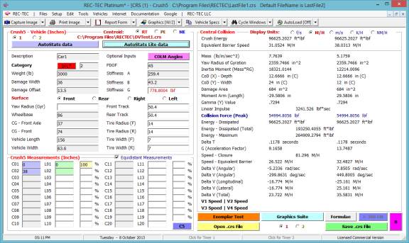
Figure 333-2

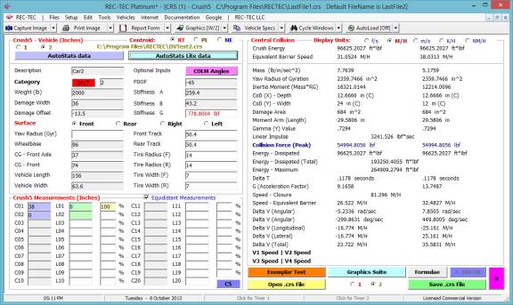
Figure 333-3 shows the Input frame for the Angles. With three angles entered, the program will display the Impact (V1 & V2) and Departure Speeds (V3 & V4) for the collision.

Note: In November of 2015, Crush5 was again upgraded to solve for the Approach angles for both V1 and V2 utilizing the Entered PDOF angles of both vehicles. This upgrade also included differentiating the Closing Velocity in a Central Collision from those in Collisions with either Module self-generated angles or User Input angles. The angles below were self-generated by the program.

Figure 333-3

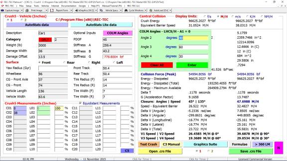
Figure 333-4

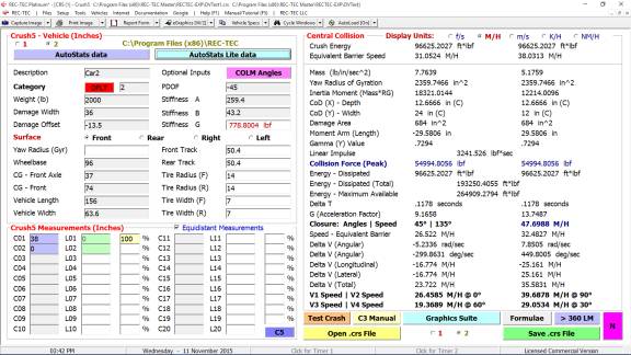
Clicking on Graphics Suite brings up Figure 333-5.

Figure 333-5

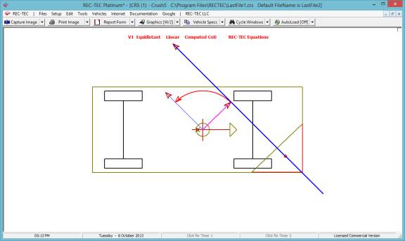
Using the Esc key (or the middle Mouse button if set to Esc) brings up Figures 333-6 through 333-9.

Figure 333-6

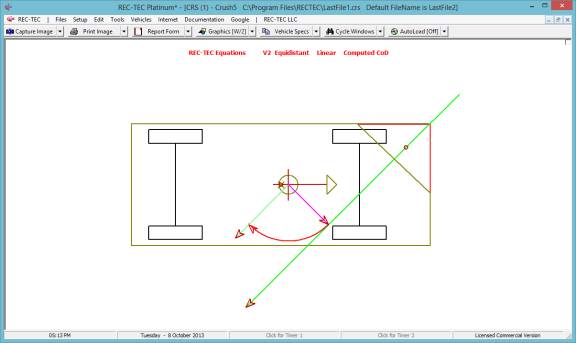
Figure 333-7

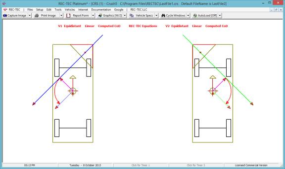
Figure 333-8

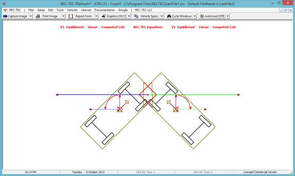
In late 2011, the CRUSHV interface was again upgraded with the inclusion of a new button [> 360 LM]. When the angles have been added and the V1, V2, V3, and V4 solutions are on the screen, this button becomes “Enabled” allowing data to be transferred from CRUSHV to the 360 Linear Momentum module. Momentum data is transferred along with the names of the .CRS Files for both vehicles. This information is immediately processed in the 360 Linear Momentum module and can be sent directly to SMAC-RT. With both the Momentum data and the Vehicle data, SMAC-RT (in REC-TEC Platinum) can properly set up the collision interface so that the Centroids of Damage are correctly positioned during the collision sequence. Figure 333-81 shows the [> 360LM] button enabled.

Figure 333-81

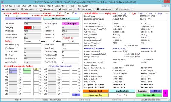
Figure 333-9

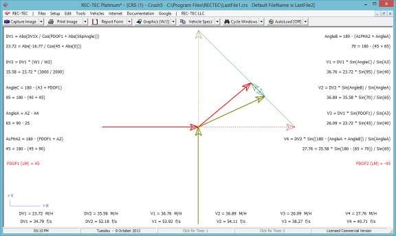
Example 2

Same data as Example 1 except A2 is Changed to 80-degrees

Figure 333-10

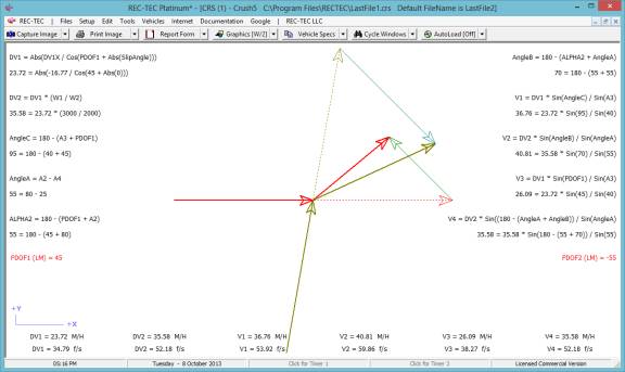
Example 3

Same data as Example 1 except A2 is Changed to 110-degrees

Figure 333-11

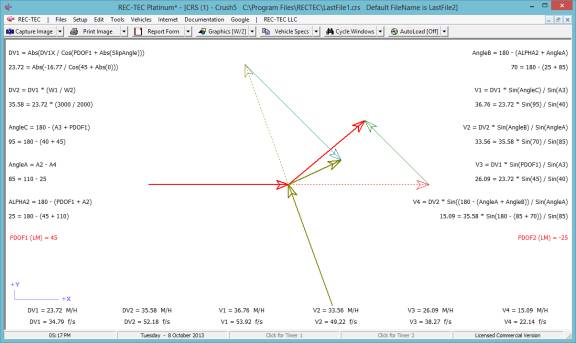
Proof of Concept – Accuracy of Non-Equidistant “C” measurements from UNDERSTANDING DELTAV FROM DAMAGE (see “Suggested Reading” at the end of this section). (Table of Contents)

Centroid of Damage (CoD)

Correct placement of the Centroid of Damage (the area center of the damage) is the single most critical part of the analysis. There are several ways to determine the Centroid of Damage. One way is to guess. This often yields remarkably good results. Another way is to use one of the published methods described below:

1. “Parkka method” reprinted from EQUATION DIRECTORY FOR THE RECONSTRUCTIONIST, by permission of the author, Daniel Parkka

Centroid of Damage is best explained utilizing two tables (see following) containing an example. Below is a frontal impact measured by utilizing six crush measurements. One profile section, C₂ to C₃, has been enlarged and the measurements have been placed into the first table. Each block of the table has been identified with a small italic constant. The large numbers, which appear in each block, are the result of mathematical equations, which are shown below the table. Each block has either an explanation or a simple mathematical formula to produce its product. This process is repeated for each crush profile section (C₁ to C₂, C₂ to C₃, C₃ to C₄ and so forth).

Figure POC-A - Enlargement of damage profile section C₂ to C₃

Crush measurements:

C₁ = 15 inches C₄ = 8 inches

C₂ = 13 inches C₅ = 5 inches

C₃ = 10 inches C₆ = 3 inches

Total damage region width (L) = 55 inches (sectioned into 5 equal segments of 11 inches)

Figure POC-B - Table 1: Damage Profile Section C₂ to C₃

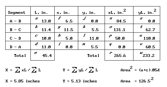
Mathematical equations or explanations for each block appear below.

a = Line AB, in m = d * 0.5

b = SQR((a-c)² + d² ) n = a * f

c = Line CD, in o = b * g

d = Line DA, in p = c * h

e = a + b + c + d, in q = d * i

f = a * 0.5 r = n + o + p + q, in²

g = (a - c) * 0.5 + c s = a * j

h = c * 0.5 t = b * k

i = Line DA in the x direction, in u = c * l

j = Line AB in the y direction, in v = d * m

k = d * 0.5 w = s + t + u + v, in²

l = Line CD in the y direction, in

The next step of this process is similar to the first utilizing a second table with the results from the first table.

NOTE: The results in crush region C₂ to C₃ below are the only ones that were processed from the previous table. C₁ to C₂ and C₃ thru C₆ are processed individually in the same manner; however, the mathematics is not shown in this example.

Figure POC-B - Table 2

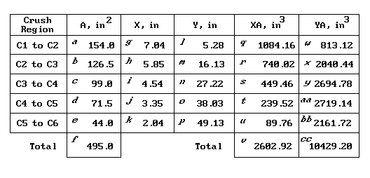
a-e = Area² of each individual crush segment taken from the first table.

f = Total area² of a-e.

g-k = Damage centroid to each individual crush profile segment in the x direction.

l-p = Damage centroid to each individual crush profile segment in the y direction.

NOTE: This distance is measured from the origin on the y-axis to the damage centroid profile.

q-u = Product of the area² and damage centroid in the x direction for each segment.

v = Total measurements of q-u.

w-bb = Product of the area² and damage centroid in the y direction variables.

cc = Total measurements of w-bb.

The centroid of damage for the entire crush region can then be located by dividing the total values of block v and cc (XA, in³ and YA, in³) by the total value of block f (A, in²).

x = 5.25 inches

(Centroid of damage in the x direction from the x and y apex over the entire length of the crush region)

y = 21.06 inches

(Centroid of damage in the y direction from the x and y apex over the entire length of the crush region)

2. “Mitchell method” from the INTERNATIONAL GUIDE BOOK for TRAFFIC ACCIDENT RECONSTRUCTION, author, J.F. Mitchell CD

The formulae currently published include the following for computing the Centroid of Damage for no more than six Equidistant or Non-Equidistant “C” measurements. These six “C” measurements define five crush “elements” or “sections.”

The Example values used in the book are:

CM(1) = 13.25 L(1) = 0

CM(2) = 11.25 L(2) = 8.5

CM(3) = 10.5 L(3) = 13.25

CM(4) = 6.25 L(4) = 16

CM(5) = 4.5 L(5) = 20.5

CM(6) = 1.5 L(6) = 25

CrushA = (L(2) - L(1)) * (CM(2) + CM(1)) * 0.5 + (L(3) - L(2)) * (CM(3) + CM(2)) * 0.5 + (L(4) - L(3)) * (CM(4) + CM(3)) * 0.5 + (L(5) - L(4)) * (CM(5) + CM(4)) * 0.5 + (L(6) - L(5)) * (CM(6) + CM(5)) * 0.5

CrushA = 216.5

Mx = CrushA * ((CM(2) + CM(1)) * 0.5) * 0.5 + CrushA * ((CM(3) + CM(2)) * 0.5) * 0.5 + CrushA * ((CM(4) + CM(3)) * 0.5) * 0.5 + CrushA * ((CM(5) + CM(4)) * 0.5) * 0.5 + CrushA * ((CM(6) + CM(5)) * 0.5) * 0.5

Mx = 1100.344

My1 = (L(2) - L(1)) * CM(1) * (L(1) + L(2)) * 0.5 + ((L(2) - L(1)) * (CM(2) - CM(1)) * 0.5 * (L(1) + (2 * (L(2) - L(1))) / 3))
My2 = (L(3) - L(2)) * CM(3) * (L(2) + L(3)) * 0.5 + ((L(3) - L(2)) * (CM(3) - CM(2)) * 0.5 * (L(2) + (2 * (L(3) - L(2))) / 3))
My3 = (L(4) - L(3)) * CM(4) * (L(3) + L(4)) * 0.5 + ((L(4) - L(3)) * (CM(2) - CM(3)) * 0.5 * (L(3) + (2 * (L(4) - L(3))) / 3))
My4 = (L(5) - L(4)) * CM(4) * (L(4) + L(5)) * 0.5 + ((L(5) - L(4)) * (CM(5) - CM(4)) * 0.5 * (L(4) + (2 * (L(5) - L(4))) / 3))
My5 = (L(6) - L(5)) * CM(5) * (L(6) + L(5)) * 0.5 + ((L(6) - L(5)) * (CM(6) - CM(5)) * 0.5 * (L(5) + (2 * (L(6) - L(5))) / 3))

My = My1 + My2 + My3 + My4 + My5

My = 1959.552

CoDX = Mx / CrushA CoDX = 5.082

CoDY = My / CrushA CoDY = 9.051

3. “Bonnett method” using the formulae currently in the REC-TEC Professional software program

CM(1) = 13.25 L(1) = 0

CM(2) = 11.25 L(2) = 8.5

CM(3) = 10.5 L(3) = 13.25

CM(4) = 6.25 L(4) = 16

CM(5) = 4.5 L(5) = 20.5

CM(6) = 1.5 L(6) = 25

For N = 1 To CrushMeasurements – 1

CrushA = CrushA + (L(N + 1) - L(N)) * (CM(N + 1) + CM(N)) * 0.5

CrushYA = CrushYA + (L(N + 1) - L(N)) * CM(N) * (L(N) + L(N + 1)) * 0.5 _

+ ((L(N + 1) - L(N)) * (CM(N + 1) - CM(N)) * 0.5 * (L(N) + (2 * (L(N + 1) - L(N))) / 3))

If CM(N) < CM(N + 1) Then

HoR = CM(N)

AreaR = CM(N) * (L(N + 1) - L(N))

Else

HoR = CM(N + 1)

AreaR = CM(N + 1) * (L(N + 1) - L(N))

End If

If CM(N) <> CM(N + 1) Then

AreaT = Abs(CM(N) - CM(N + 1)) * (L(N + 1) - L(N)) * 0.5

CrushXA = CrushXA + (HoR + 2 * Abs(CM(N) - CM(N + 1)) / 3) * AreaT _

+ (HoR + Abs(CM(N + 1) - CM(N)) * 0.5) * AreaR

Else

CrushXA = CrushXA + HoR * AreaR

End If

Next

CrushXA = CrushXA * 0.5 CrushA = 216.5

CrushX = 927.5078

CoDX = CrushX / CrushA CoDX = 4.2841

CrushY = 2065.5260

CoDY = CrushY / CrushA CoDY = 9.5405

Compare these values with Mitchell’s example. The other difference between the Bonnett and Mitchell formulae is that the Mitchell formulae limit the user to a 6-point or less examination of the damaged area while the Bonnett formulae have no reasonable limit on the number of “C” measurements. REC-TEC software allows for up to 20 “C” measurements in the computations for Centroid of Damage and CRUSH.

So Which Witch is Which?

In order to determine which of these 3 different methodologies is correct, it is necessary to actually plot the points in a damage area. In order to do this efficiently, REC-TEC employs vehicle files that incorporate some very specific damage. The “damage” is not “real-world damage.” It is a geometric shape that will enable quick visual confirmation that the graphics are operating correctly and that the formulae are generating correct information. Using the Geometric approach allows those of us not having advanced mathematical degrees after our name to demonstrate the accuracy of the approach.

Basically, almost any vehicle measurements can be used. What is important is the shape of the damage. In the tests both a “rectangular” and a “triangular” shape are used, as the represent the main challenges for the algorithm. These shapes tend to exacerbate any errors in the calculation of the Centroid of Damage. One of the vehicles has Equidistant “C” measurements and the other has Non-Equidistant “C” measurements. This also will verify that these two methods (Equidistant / Non-Equidistant) generate similar values.

Equidistant Non Equidistant

For the “Rectangular” shape, the following values are used.

CM(1) = 15 CM(1) = 15 L(1) = 0

CM(2) = 15 CM(2) = 15 L(2) = 5

CM(3) = 15 CM(3) = 15 L(3) = 10

CM(4) = 15 CM(4) = 15 L(4) = 15

CM(5) = 15 CM(5) = 15 L(5) = 60

For the “Triangular” shape, the following values are used.

CM(1) = 0 CM(1) = 0 L(1) = 0

CM(2) = 12 CM(2) = 5 L(2) = 5

CM(3) = 24 CM(3) = 10 L(3) = 10

CM(4) = 36 CM(4) = 15 L(4) = 15

CM(5) = 48 CM(5) = 20 L(5) = 20

CM(6) = 60 CM(6) = 60 L(6) = 60

The following graphics screens will show each of the methodologies described above and should be self-explanatory. All of the graphics were generated using REC-TEC Professional software.

The practical effect may not be as drastic as the graphics may imply. The error is 1 to 3 miles per hour in most normal damage configuration accidents. The further the geometric shape is removed from that of a square, the closer the “Parkka” equations are to correct. The “Mitchell” equations are simply incorrect as published.

Example 1

Figure POC-C – Parkka: Error on Non-Equidistant (PDOF)

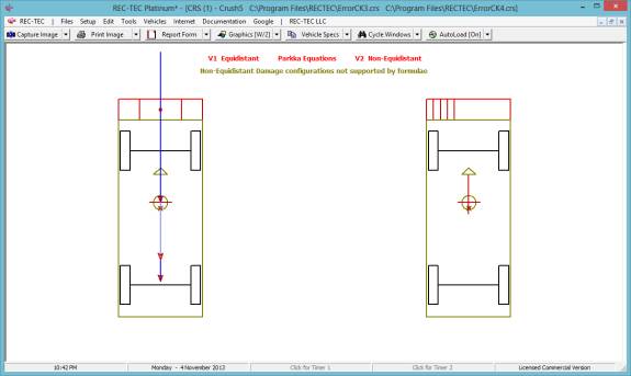
Figure POC-D – Mitchell: Correct – Depths equal, C1=C2=C3=C4

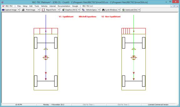
Figure POC-E – Bonnett/REC-TEC: Correct – Depths equal, C1=C2=C3=C4

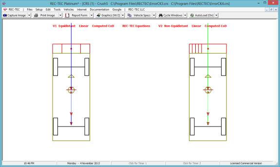
Example 2

Figure POC-F – Parkka: Error on Non-Equidistant (PDOF)

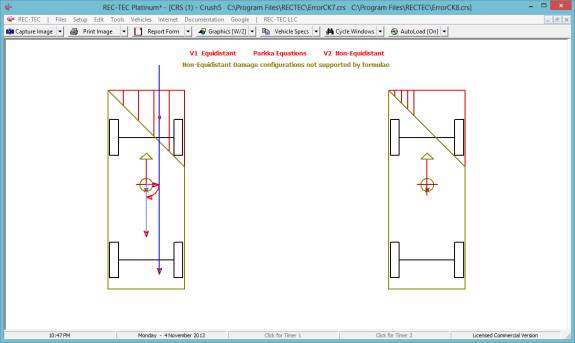
Figure POC-G – Parkka: Vehicle 1

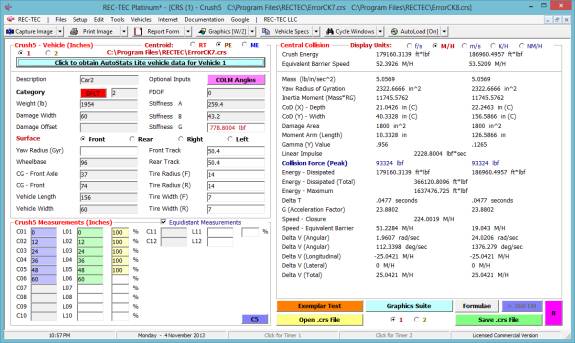
Check Centroid of Damage (CoD) and DeltaV (Angular) data Formulae does not support V2 “L” data

Figure POC-H – Parkka: Vehicle 2

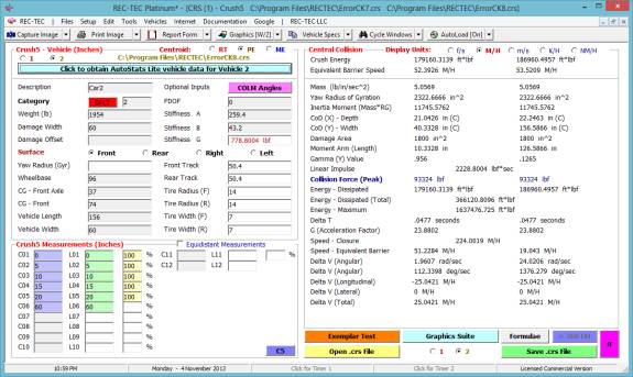
Figure POC-I – Mitchell

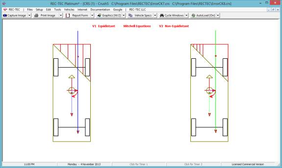
Both Vehicle Diagrams appear correct but check the Centroid of Damage (CoD) data Error in CoD

Figure POC-J – Mitchell: Vehicle 1

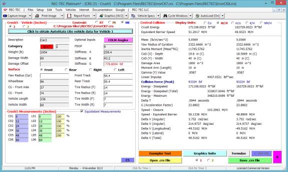
Figure POC-K – Mitchell: Vehicle 2

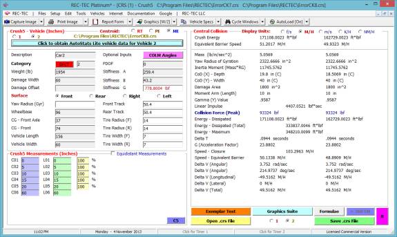
Triangle CoD for side (not hypotenuse) is side (60) divided by 3 20 or 40 correct depending on start

Figure POC-L – Bonnett/REC-TEC

Figure POC-M – Bonnett/REC-TEC: Vehicle 1

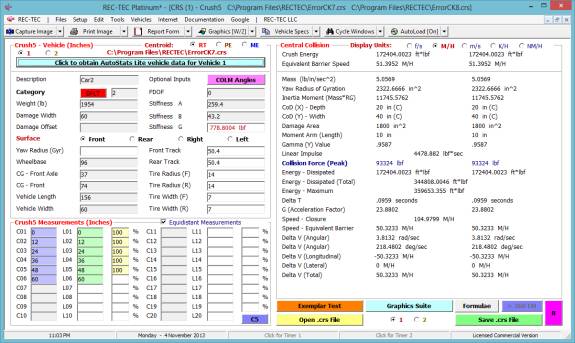
Compare Bonnett (RT) Centroid of Damage (CoD) data with Mitchell and Parkka 60/3 = 20 (or 40)

Figure POC-N – Bonnett/REC-TEC: Vehicle 2

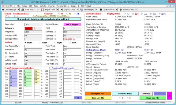
Example 3

Figure POC-O – Parkka

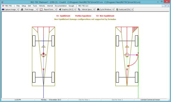
The PDOF should be on centerline and the CoD on the tip of the yellow arrowhead as shown on Bonnett/REC-TEC (POC-Q)

Figure POC-P – Mitchell

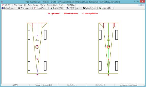
Figure POC-Q – Bonnett/REC-TEC

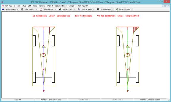
Suggested reading for additional information:

· CRASH3 Technical Manual – Internet

· IPTM Publications – The following publications are available from IPTM 1-904-620-4786 or http://www.iptm.org and are recommended for further reading.

o ANATOMY of a COLLISION by George M. Bonnett contains an article entitled Stiffness Coefficients – Energy and Damage, detailing stiffness coefficients. The book also contains both of the below listed articles.

o UNDERSTANDING DELTAV FROM DAMAGE – Discussion includes Crash3 formulae and computations for non-equidistant "C" measurements.

o BEYOND CRASH3 – DELTAV FROM DAMAGE – Discussion of depth "zones" for non-linear crush and modeling of bullet-shaped or curved vehicles.

Module 30: Energy - Damage Analysis > Crush (Vomhof)

(Table of Contents)

Overview: This module computes “Kinetic Energy Equivalent Speed” or “Closing Speed” of collision using the Vomhof (4N6XPRT SYSTEMS) methodology employing “Crush Factors.”

At the REC-TEC pull down menu, select Energy - Damage Analysis > Crush (Vomhof) and the Crush (Vomhof) screen appears (Figure 334).

Figure 334

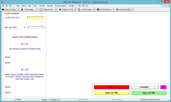
Required Input Data

· Crush Factor (CF) – Not a “Stiffness Coefficient” - See Notes below

· Max. Ind. Dpth. – Maximum Indentation Depth - See Notes below

· Note 1: Default CF values are based upon analysis of NHTSA Barrier Crash data, and from over 1000 vehicle accidents where independent evaluation of speed was possible. (These are NOT 'A', 'B', 'C', or 'G' values.)

· Note 2: Rear impact data with more than 2 to 3 inches of crush damage should be looked at carefully, since some vehicles have very weak trunk and fender strength. Therefore, on some cars, especially GM, your estimate from the rear crush data may be high by as much as 4 to 5 mph on a crush of 18 inches.

· Note 3: Crush Factor (CF) = 21. This value is used in place of the drag factor when you have information on other post impact speeds. The speed calculated can be COMBINED with other crush speeds and post impact speeds. This DOES NOT calculate a delta-V. It calculates the energy to create the crush, expressed as a speed.

· Note 4: Crush Factor (CF) = 27. This value is used in place of the drag factor in the minimum speed from skid formula. The 27 is used when you have the target vehicle, and no other information post impact (speeds, positions, skids, etc), but you have to come up with SOMETHING for speed of the bullet vehicle. The speed calculated CANNOT be combined with other subsequent crush speeds and post impact speeds. This DOES NOT calculate a delta-V. It calculates the IMPACT SPEED for the BULLET vehicle based upon the TARGET vehicle damage ONLY. To work, you must have good, solid impact between bullet and target vehicles, not a glancing blow.

Example 1: The crush depth is 15 inches and the Crush Factor is 21.

Figure 335

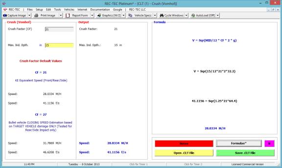
Example 2: The crush depth is 15 inches and the Crush Factor is 27.

Figure 336

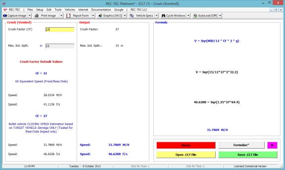
Module 31: Energy - Damage Analysis > Reduced Mass (CEES)

(Table of Contents)

Overview: This module computes the “Reduced Mass” of vehicles in collision and the maximum and actual Energy available for Damage and relative Translational Motion. It also computes the Crush Energy Equivalent Speed (CEES) for the collision.

At the REC-TEC pull down menu, select Energy - Damage Analysis > Reduced Mass (CEES) and the Energy–Reduced Mass screen appears (Figure 337).

Figure 337

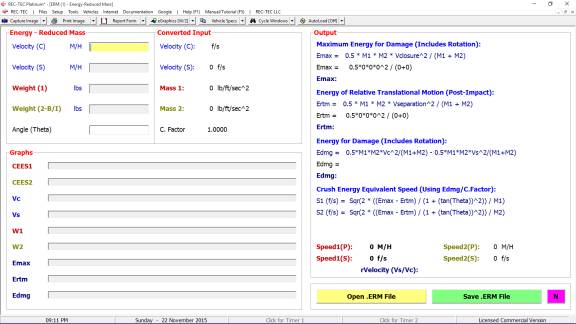
Required Input Data

· Velocity (C) – Closing Velocity

· Velocity (S) – Separation Velocity

· Weight (1) – Weight of Unit 1 in Test Crash

· Weight (2-B/I) – Weight of Unit 2 (Barrier/Impactor) in Test Crash

· Angle (Theta) – The angle between the PDOF and a line Perpendicular to the Surface Struck

Additional Information: The IPTM publication, Anatomy of a Collision by George M. Bonnett contains an article entitled Stiffness Coefficients – Energy and Damage, detailing this process and is recommended for further reading. 1-904-620-4786 or http://www.iptm.org

Example 1: A crash test involved an impactor (4000#) moving at 30 M/H, which struck a stationary Target vehicle (2750#) in the side at an angle of zero degrees relative to an angle perpendicular to the surface struck. No post-impact data was reported. The vehicles remained together after impact.

What impact speed should be entered into the computations for the A and B stiffness coefficients?

Does it make a difference if the impactor is moving, or the vehicle is moving with a stationary impactor?

Figure 338

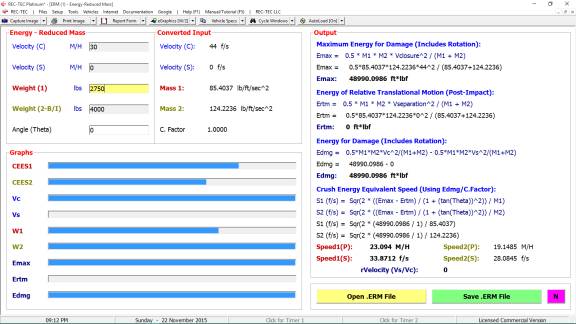
Example 2: Use the same information as for Example 1 except that the angle is 45 degrees.

What impact speed should be entered into the computations for the A and B stiffness coefficients?

Figure 339

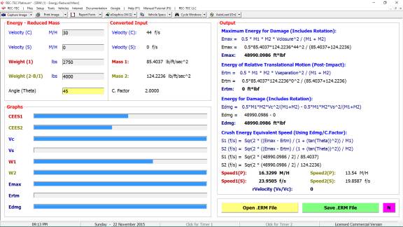
The answers in this module will be examined in Module 32.

Module 32: Energy - Damage Analysis > Stiffness Coefficients

(Table of Contents)

Overview: This module computes A, B, and G Stiffness values using data obtained from car-barrier or car-impactor collisions.

At the REC-TEC pull down menu, select Energy - Damage Analysis > Stiffness Coefficients and the Stiffness Coefficients screen appears (Figure 340).

Figure 340

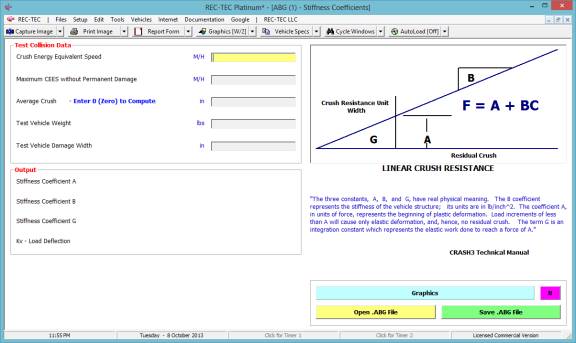
Required Input Data

· Crush Energy Equivalent Speed – Exemplar Vehicle in Test Crash

· Maximum CEES without Permanent Damage

· Average Crush – Enter 0 (Zero) to Compute

1. Number of “C” Measurements

2. Length of (Each) “C” Measurement

· Test Vehicle Weight – Exemplar Vehicle in Test Crash

· Test Vehicle Damage Width – Exemplar Vehicle in Test Crash

Example 1: Crush Energy Equivalent Speed is 23.094 M/H. Maximum Speed without damage = 2 M/H. Average Crush is 20 inches. Test vehicle weight is 2750 lbs. Test vehicle damage width is 72 inches.

Figure 341

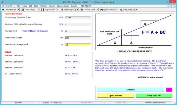
Example 2: Crush Energy Equivalent Speed is 16.3299 M/H. Maximum Speed without damage = 2 M/H. Average Crush is 20 inches. Test vehicle weight is 2750 lbs. Test vehicle damage width is 72 inches.

Figure 342

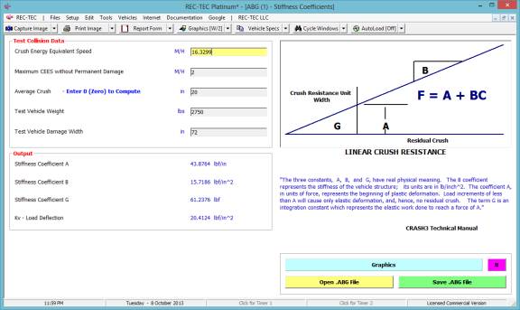
Example 3: Closing Speed is 30 M/H. Maximum Speed without damage = 2 M/H. Average Crush is 20 inches. Test vehicle weight is 2750 lbs. Test vehicle damage width is 72 inches.

Figure 343

The test crash (Module 31 – Figure 338 – Example 1) involved an impactor and target vehicle with a closing speed of 30 M/H. No post-impact data was reported. The impactor and the vehicle traveled for some distance post-impact, but no distances were recorded. The only kinetic energy brought into the collision was from the moving impactor. This energy was primarily converted into both damage and translational motion of the impactor and the vehicle. Target vehicles are not placed against an immovable barrier when being struck by an impactor; it is free to move after being struck by the impactor.

Since no measurements were made of the post impact motion, how can the energy that went into translational motion be computed? Obviously, not all of the energy went into damage. In CRUSHV (Module 29 – Figure 312 – Example 1) the Aston Martin had an EBS of 29.9999, but in Module 29 – Figure 321 – Example 2) the total DeltaV for the Aston Martin was only 24.4025 M/H. with the same damage and caused a 40.0518 M/H DeltaV to the other (lighter) vehicle which had been stopped. There is a problem, but the Reduced Mass computations in Module 31 provide a solution.

Another solution is available from 4N6XPRT Systems. Their solution is called KEES (Kinetic Energy Equivalent Speed). KEES uses an entirely different approach that arrives at exactly the same solution. Contact 4N6XPRT Systems at http://www.4N6XPRT.com for additional information on their paper.

Module 33: Miscellaneous – Rotation Factor

(Table of Contents)

Overview: This module computes an approximate deceleration adjustment factor for a vehicle in rotation.

At the REC-TEC pull down menu, select Miscellaneous > Rotation Factor and the Rotation Factor screen appears (Figure 344).

Figure 344

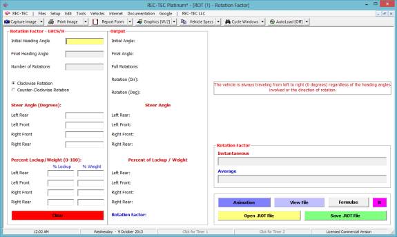
Required Input Data

· Initial Heading Angle – Vehicle is always traveling Left to Right (0 Degrees)

· Final Heading Angle – Vehicle is always traveling Left to Right (0 Degrees)

· Number of Rotations – Number of Complete Rotations

(Button) Clockwise Rotation

(Button) Counter-Clockwise Rotation

Steer Angle (Degrees):

· Left Rear – Steer Angle of Wheel

· Left Front – Steer Angle of Wheel

· Right Front – Steer Angle of Wheel

· Right Rear – Steer Angle of Wheel

Percent Lockup/Weight (0-100):

· Left Rear – % Lockup / % Weight

· Left Front – % Lockup / % Weight

· Right Front – % Lockup / % Weight

· Right Rear – % Lockup / % Weight

Example 1: A vehicle has an initial heading angle of 45 degrees and a final heading angle of 315 degrees after going through 3 complete rotations in a clockwise direction. There are no steer angles and there is no braking. The weight is identical on all wheels.

Figure 345

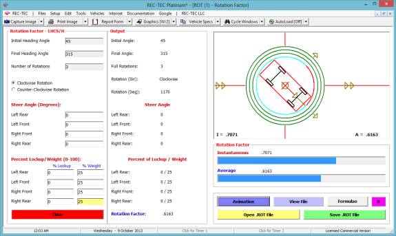
Example 2: Modify Example 1 to include a slip angle on the front wheels of 15 degrees, front brakes that were developing 30 % braking, and rear wheels that were developing 20% braking.

Figure 346

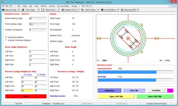
Example 3: Modify Example 2 to include no full rotations.

Figure 347

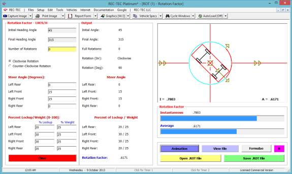
Figure 348

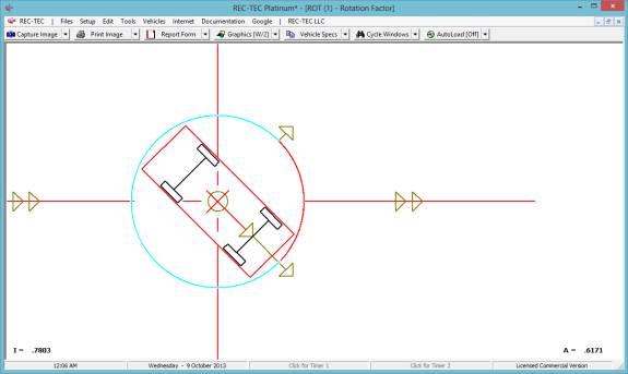
Example 4: Using the data in Example 3, a vehicle decelerates to a stop in 75 feet on a 0.75 surface.

What was the initial speed of the vehicle?

Solution 1: Multiply 0.75 by the rotation factor of 0.6171 (Figure 349).

Figure 349

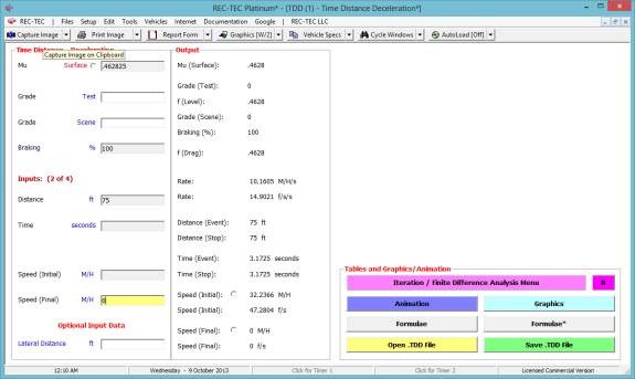
Solution 2: Use 0.75 as the Surface Friction or Mu and use the rotation factor of 0.6171 (multiplied by 100) as the percent of braking (Figure 350).

Figure 350

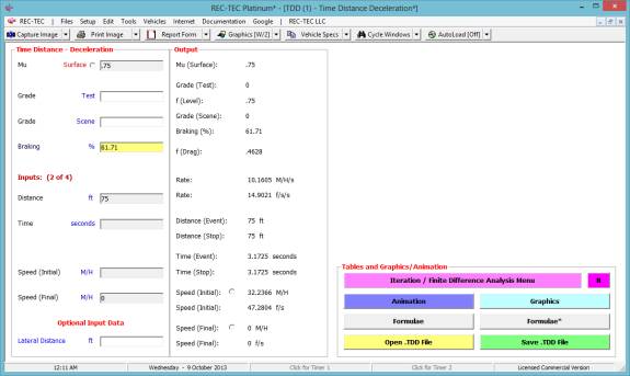
Either solution results in the same result, 32.2366 M/H.

Figure 351 shows the beginning of the file including the formulae used, which was automatically created for the rotation in Figure 347. Figure 352 shows the end of the file.

Figure 351

Figure 352

Module 34: Miscellaneous – Speed - Hydroplane

(Table of Contents)

Overview: This module computes the speed at which a tire will hydroplane using published formula under various (input) conditions.

At the REC-TEC pull down menu, select Miscellaneous > Speed - Hydroplane and the Speed - Hydroplane screen appears (Figure 353).

Figure 353

Required Input Data

· Air Pressure (PSI) – Tire Air Pressure (PSI) – Navin: (Range 16-36 PSI)

(Button) Normal Wear

(Button) Bald Tires

· Aspect Ratio – Tire Footprint (Width/Length) – Navin: (Range .6 - 1.4)

If Aspect Ratio Unknown Use

· Width – Width of Tire Footprint

· Length – Length of Tire Footprint

If Length Unknown Use

· H. Diameter – Horizontal Diameter of Tire

· V. Diameter – Vertical Diameter of Tire

Example 1: A vehicle has tires with normal wear and air pressure of 35 pounds of air. The horizontal diameter of the tires is 29 inches and the vertical diameter is 28.25 inches.

What is the Aspect Ratio?

At what speed will the vehicle hydroplane?

Figure 354

If the vehicle has bald tires, what changes?

Figure 355

Notice that in addition to a change in the speeds, the NASA Spin-Down formula was replaced with the NASA Spin-Up formula, and yes, NASA does refer to the National Aeronautics and Space Administration.

Figure 356 displays the Finite Difference Analysis for the NASA Spin-Up formula.

Figure 356

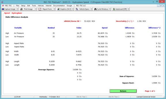
Figure 357 displays the Finite Difference Analysis for the Navin formula.

Figure 357

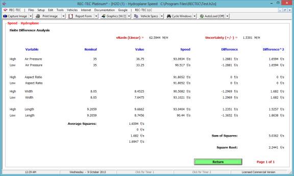
Module 35: Miscellaneous – Speed - RPM

(Table of Contents)

Overview: This module computes the Speed of a vehicle or bicycle based on engine speed and two gear ratios.

At the REC-TEC pull down menu, select Miscellaneous > Speed - RPM and the Speed - RPM screen appears (Figure 358).

Figure 358

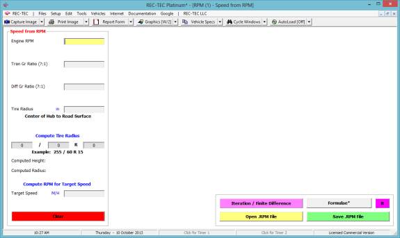
Required Input Data

· Engine RPM – RPM of the Engine

· Tran Gr Ratio (?:1) – Transmission Gear Ratio (N:1)

· Diff Gr Ratio (?:1) – Differential Gear Ratio (N:1)

· Tire Radius – Center of Hub to Road Surface

Optional Inputs

· Tire Radius – Tire Width, Profile, and Rim Diameter (255/60R15) used to compute Sidewall height and Radius.

· Target Speed – Target speed used to compute the required RPM based on available input information

Note – Module will show formula for speed or RPM as appropriate using Formulae* button

Example 1: A vehicle with a rolling radius on the drive wheels of 15 inches, a differential gear ratio of 4.11:1, and a transmission final gear ratio of 1:1 is running at 5000 rpm.

What is the speed of the vehicle?

Figure 359

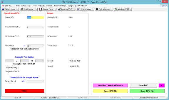
Figure 359B

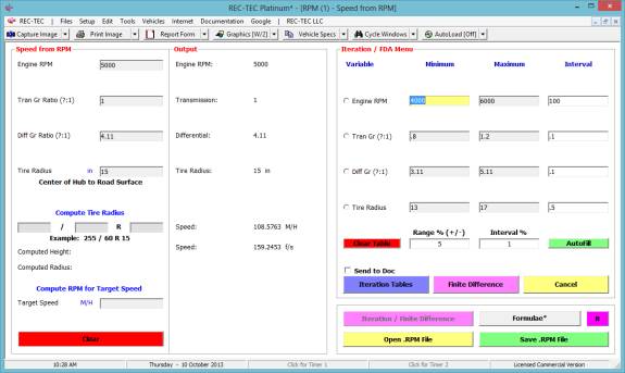
Using the data in Figure 359B, generate a table based on the range of the Engine RPM.

Figure 359C

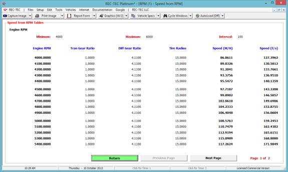
Figure 359D

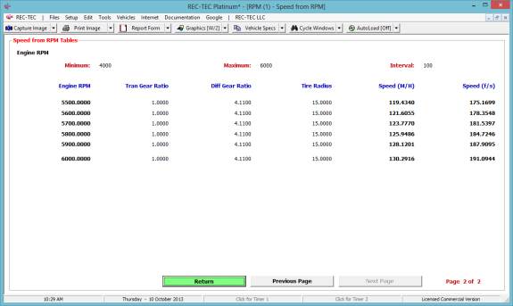
Using the data in Figure 359B, generate a table based on the range of the Tire Radius.

Figure 359E

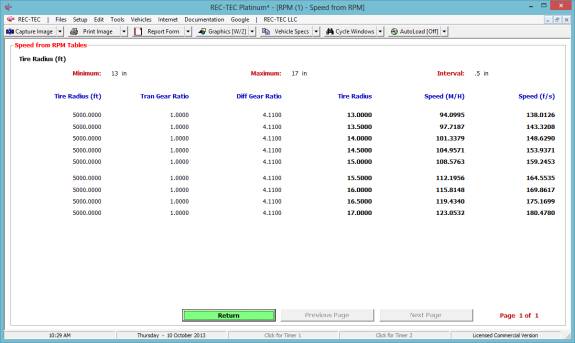
Using the data in Figure 359B, generate the Finite Difference Analysis.

Figure 359F

Example 1A: Using the data in Example 1, if the original tires generated a speed of 60 M/H, how would replacing those tires change the speed of the vehicle with the same wheel speed?

Figure 359G

Figure 359H

With an RPM of 2763.0316 we then show a range of Tire Radii of 2 inches either side of the 15 inch original tires in Figure 359I. The speed range is from 52 to 68 miles per hour depending on the Tire radius.

Figure 359I

Example 1B: What is the Tire RPM, the Tire radius, and Height for a 225/60R16 tire at 60 M/H?

Figure 359J

The Wheel RPM and the Engine RPM are the same with both gear ratios at 1:1.

Example 2: A cyclist with a cadence of 90 RPM is on a bicycle with 28 diameter tires. The front chain ring has 50 teeth and the rear has 13 teeth.

What is the speed of the cyclist?

Figure 360

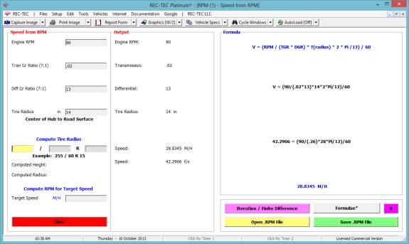
Transmission = 1:50 = 1/50 = 0.02:1 Differential = 13:1 Radius = Diameter/2

Module 36: Miscellaneous – Tangent Offset

(Table of Contents)

Overview: This module computes Tangent Offset information.

At the REC-TEC pull down menu, select Miscellaneous > Tangent Offset and the Tangent Offset screen appears (Figure 361).

Figure 361

Required Input Data

· Chord: – Chord if known (Unit independent – Use same units for all inputs)

+

· Middle Ordinate: – Middle Ordinate (Unit independent)

OR

· Radius: – Radius if known (Unit independent – Use same units for all inputs)

· Paper Length: – Scale Diagram

· Scene: – Used to determine Scale if Scene is larger than Tangent Length

· Tangent Length: – Used to determine Scale

· Interval: – Along X-Axis (Baseline)

Example 1: A yaw mark has a chord of 50 feet and a middle ordinate of 3 feet. The drawing must fit on a standard size page (11 inches) and the scene is 100 feet long. An interval of 5 feet will suffice.

What are the X and Y points for the yaw?

What is the maximum scale to fit the page (include units)?

Figure 362

Module 37: Miscellaneous – Weight Shift (3-Axis)

(Table of Contents)

Overview: This module computes Passenger Vehicle, Straight Truck, Bus or other non-articulated Vehicles three-dimensional center of gravity based on information about vehicle and weights on the wheels when level and then raised. This module will also compute rollover speeds and critical speed of curve data.

At the REC-TEC pull down menu, select Miscellaneous > Weight Shift (3-Axis) and the Weight Shift (3-Axis) screen appears (Figure 363).

Figure 363

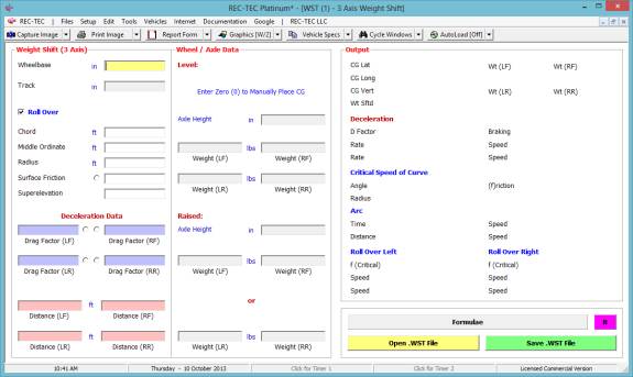
Required Input Data

· Wheelbase – Vehicle Wheelbase

· Track – Vehicle Track

· Chord – Required with Middle Ordinate

· Middle Ordinate – Required with Chord

OR

· Radius – Radius of Curve

· Mu – Surface Friction

· Superelevation – Tangent of Angle (Adjustment in direction of Striation Marks)

Deceleration Data:

· Drag Fctor (LR) – Drag Factor corrected for grade

· Drag Fctor (LF) – Drag Factor corrected for grade

· Drag Fctor (RF) – Drag Factor corrected for grade

· Drag Fctor (RR) – Drag Factor corrected for grade

Distance:

· Distance (LR) – Deceleration Distance of Wheel

· Distance (LF) – Deceleration Distance of Wheel

· Distance (RF) – Deceleration Distance of Wheel

· Distance (RR) – Deceleration Distance of Wheel

Level: (Enter Zero (0) to Manually Place CG)

· Axle Height – Level (Measured from Surface)

· Weight (LR) – Weight on Wheel when Level

· Weight (LF) – Weight on Wheel when Level

· Weight (RF) – Weight on Wheel when Level

· Weight (RR) – Weight on Wheel when Level

Raised: (Enter Zero (0) to Manually Place CG)

· Axle Height – Raised (Minimum of 30 inches)

· Weight (LF) – Weight on Wheel when Rear Axle Raised

· Weight (RF) – Weight on Wheel when Rear Axle Raised

OR

· Weight (LR) – Weight on Wheel when Front Axle Raised

· Weight (RR) – Weight on Wheel when Front Axle Raised

Manual Placement of CG

· Vertical – CG Vertical from Road Surface

· Lateral – CG Lateral (from Left)

· Longitudinal – Longitudinal (from Rear Axle)

· Vehicle Weight – Total Weight of Vehicle

Example 1: Figure 364 is an example of a 3-Axis Weight Shift problem including both the inputs and outputs from the module.

Figure 364

Module 38: Railroad Grade Crossings – AASHTO/AREA Vertical Alignment

(Table of Contents)

Overview: This module computes compliance of on-grade crossings with the requirements of AASHTO/AREA standards.

At the REC-TEC pull down menu, select Railroad Grade Crossings > AASHTO/AREA Vertical Alignment and the AASHTO/AREA Vertical Alignment screen appears (Figure 365).

Figure 365

Required Input Data

· Right Rail Elevation Change – From Left Rail (+/-)

· Right Approach Elevation Change – Measured from Right Rail at a distance of 30 feet.

· Left Approach Elevation Change – Measured from Left Rail at a distance of 30 feet.

Example 1: The right rail elevation is –1 inch. The right approach elevation change at 30 feet is 1.5 inches. The left approach elevation change at 30 feet is -3 inches.

Figure 366

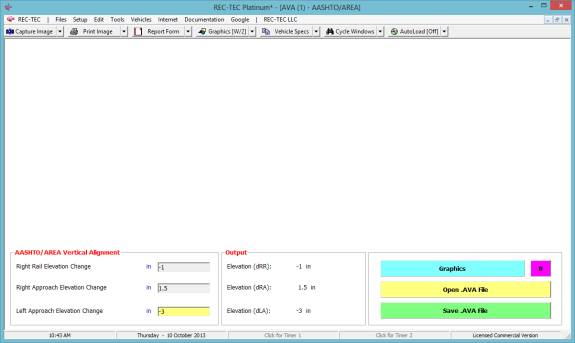
Figure 367

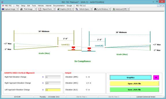
Example 2: The right rail elevation is 1 inch. The right approach elevation change at 30 feet is 1.5 inches. The left approach elevation change at 30 feet is -5 inches.

Figure 368

Figure 369

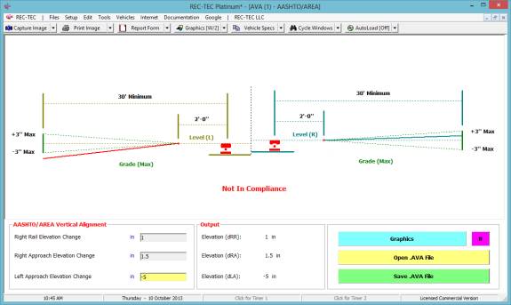
Module 39: Railroad Grade Crossings – AASHTO Sight Triangle

(Table of Contents)

Overview: This module computes the required Sight Triangle values at on-grade railroad crossings.

At the REC-TEC pull down menu, select Railroad Grade Crossings > AASHTO Sight Triangle and the AASHTO Sight Triangle screen appears (Figure 370).

Figure 370

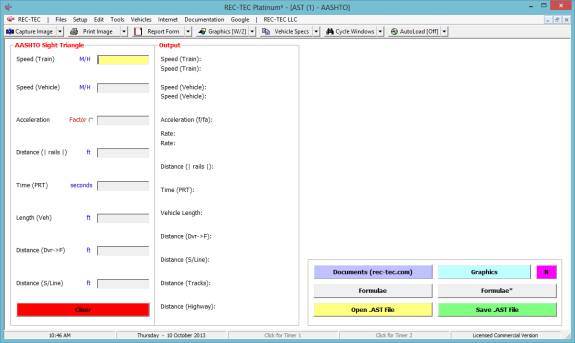
Required Input Data

· Speed (Train) – Rail Speed

· Speed (Vehicle) – Posted Speed Limit

· Acceleration – Acceleration or Deceleration (required)

· Distance (| rails |) – Distance between Outer Rails

· Time (PRT) – Perception Reaction Time (See Formulae)

· Length (Veh) – Overall Length of Vehicle

· Distance (Dvr->F) – Distance from Driver to Front of Vehicle

· Distance (S/Line) – Distance from Stop Line to First Rail

RAILROAD - HIGHWAY GRADE CROSSING HANDBOOK (FHWA-TS-86-215)

TRAIN VELOCITY assumed to be RAIL VELOCITY/SPEED.

VEHICLE VELOCITY/SPEED assumed to be POSTED LIMIT.

ACCELERATION FACTOR assumed to be 1.47 F/S^2 OR F= .045.

MAXIMUM ATTAINABLE VELOCITY assumed to be 8.8 F/S OR 6 M/H.

DECELERATION FACTOR:

10 M/H = .40 20 M/H = .40 30 M/H = .35 40 M/H = .32

50 M/H = .30 60 M/H = .29 70 M/H = .28

RAIL TO RAIL DISTANCE assumed to be 5 feet for SINGLE TRACK.

PRT (APPROACHING) assumed to be 2.5 seconds.

PRT (STARTUP) assumed to be 2 seconds.

VEHICLE LENGTH assumed to be 65 feet.

DRIVER TO FRONT OF VEHICLE DISTANCE assumed to be 10feet.

STOP LINE TO FIRST RAIL DISTANCE assumed to be 15 feet.

Example 1: A 65 ft. vehicle approaches a railroad crossing at 45 M/H and a train is traveling at 60 M/H. The drag factor of the road is 0.6. The PRT is 2 seconds. The distance between outer rails is 5 feet. The distance from front of vehicle to first rail is 15 feet. The distance from front of vehicle to driver is 10 feet.

What are the sight triangle distances?

Figure 371

Figure 372 displays the Graphics indicating the sight lines from Figure 371.

Figure 372

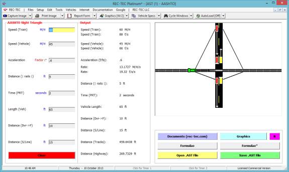
Example 2: Another vehicle that is 18 feet long is stopped at the stop line (15 feet). This vehicle is capable of accelerating to a maximum speed of 25 M/H with an acceleration factor of .25 in first (low) gear. Using the basic information in Example 1 with the modifications given here, compute the required AASHTO Track distance.

Figure 373

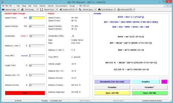
Figure 374 displays the Graphics indicating the sight lines from Figure 373.

Figure 374

Module 40: Railroad Grade Crossings – Electronic Rail Circuits

(Table of Contents)

Overview: This module displays graphically the operation of Electronic Rail Circuits.

At the REC-TEC pull down menu, select Railroad Grade Crossings > Electronic Rail Circuits and the Electronic Rail Circuits screen appears (Figure 375).

Figure 375

Required Input Data

· Train 1 [Green] Speed: – Speed of Train 1

· Train 2 [Blue] Speed: – Speed of Train 2

Graphics – Displays an interactive graphic showing the Electronic Rail Circuit for a Railroad Grade Crossing. The graphic shows and describes the Approach and Island Circuits as well as the status of the Signals. Trains are moved using Drag/Drop. As the Trains are moved into different positions, the Signals are shown to be Active or Inactive as discussed in the descriptions for the Speeds Entered.

This module can be used for Show and Tell to assist in describing the functionality of the approach and rail circuits. The Trains (upper or lower) may be moved using Drag and Drop.

Example 1: Train 1 speed is 25 M/H. Train 2 speed is 3 M/H. Neither train has entered the circuits.

Figure 376

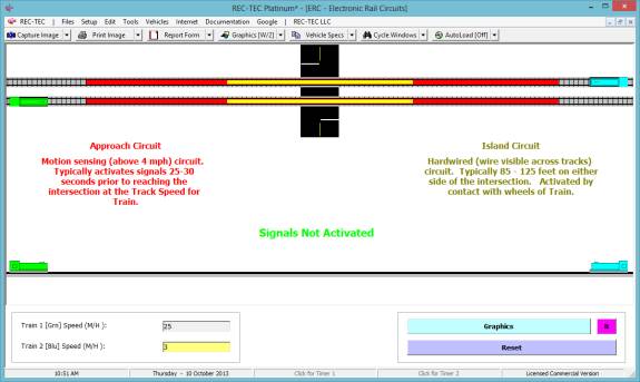
Example 2: Train 1 speed is 25 M/H. Train 2 speed is 3 M/H. Blue Train is in the Approach Circuit.

Figure 377

Example 3: Train 1 speed is 25 M/H. Train 2 speed is 3 M/H. Green Train is in the Approach Circuit.

Figure 378

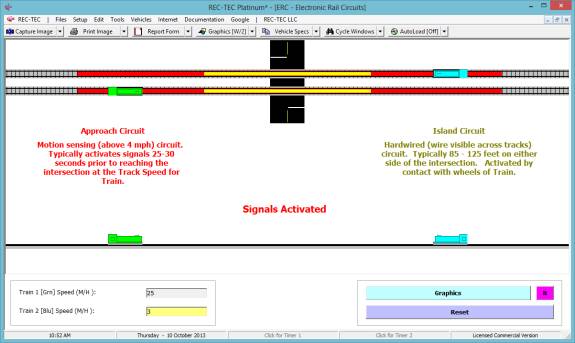
Example 4: Train 1 speed is 25 M/H. Train 2 speed is 3 M/H. Blue Train is in the Approach Circuit. Green Train has exited the Island Circuit.

Figure 379

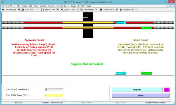
Module 41: Combined Speed Formula

(Table of Contents)

Overview: This module uses the formula Sqr (a^2 + b^2 + c^2…) to combine the entries. It can be used for speeds, solving for the hypotenuse of a right triangle, or any other numbers that must be combined in this manner.

At the REC-TEC pull down menu, select Combined Speed Formula and the Combined Speed Formula screen appears (Figure 380).

Figure 380

Required Input Data

· Number of Entries (Max = 15)

· Entry (1 through Number of Entries)

· Minimum Speed Calculation

1. Drag Factor

2. Distance

Example 1: A Right Triangle has the two sides adjacent to the right angle that measure 3 and 4 respectively.

How long is the Hypotenuse?

Figure 381

Example 2: If computed individually, the separate “decelerate to a full stop” speeds for the three different surfaces were 31.0725 M/H, 19.728 M/H, and 22.0226 M/H.

How fast was the vehicle going at the start of the maneuver?

Figure 382

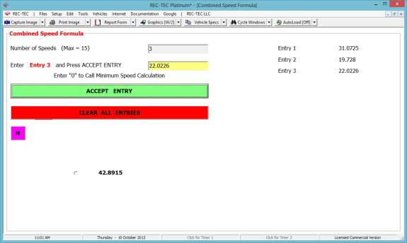
Compare this answer with that in Module 18, Example 2, Figure 187.

Module 42: Conversions

(Table of Contents)

Overview: This module does most of the conversions used in AR.

At the REC-TEC pull down menu, select Conversions and the Conversions screen appears (Figure 383).

Figure 383

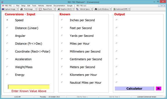
Required Input Data

Button to select:

· Speed

· Linear

· Angular

· Distance

· Coordinate

· Acceleration

· Weight /Mass

Button to select:

· Known – Select Known measurement from list (Dependent upon initial selection above)

Text Block(s) – Enter known value for measurement

Example 1: A bicycle tire has a diameter of 700 millimeters.

What is the diameter in inches?

Figure 384

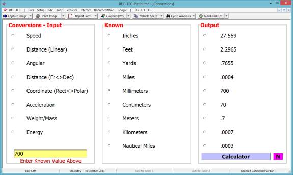
Example 2: A drag factor was determined to be 1.0

What is the rate in meters/second/second?

Figure 385

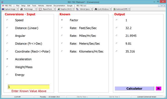
Module 43: Quadratic Solver

(Table of Contents)

Overview: This module computes the real and imaginary roots of a quadratic equation.

At the REC-TEC pull down menu, select Quadratic Solver and the Quadratic Solver screen appears (Figure 386).

Figure 386

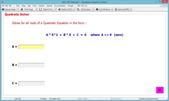
Solves for all roots of a Quadratic Equation in the form:

A * X^2 + B * X + C = 0 where A <> 0 (zero)

Required Input Data

· A = (Textbox) – Enter value for A

· B = (Textbox) – Enter value for B

· C = (Textbox) – Enter value for C

Example 1: A = 5, B = 3, and C = -1

Are the roots real or imaginary?

What are the roots?

Figure 387

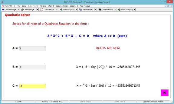
Example 2: A = 5, B = 3, and C = 1

Are the roots real or imaginary?

What are the roots?

Figure 388

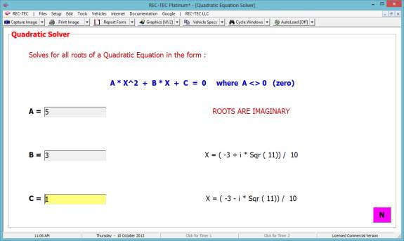
Module 44: Triangle Solver

(Table of Contents)

Overview: This module computes detailed information on a Triangle defined by three sides or side/angle information.

At the REC-TEC pull down menu, select Triangle Solver and the Triangle Solver screen appears (Figure 389).

Figure 389

Required Input Data

Triangle Solver – Input (3 of 6)

· Angle a – Angle opposite Side A

· Angle b – Angle opposite Side B

· Angle c – Angle opposite Side C

Three angles are not allowed

· Side A – Side opposite Angle a

· Side B – Side opposite Angle b

· Side C – Side opposite Angle c

Three sides are allowed

Example 1: A = 3, B = 4, and C = 5

Describe this angle.

What is the perimeter?

Figure 390

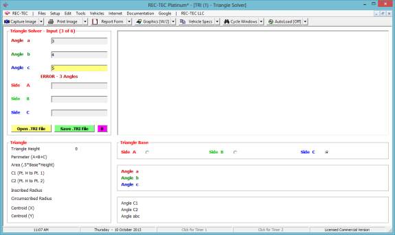
Figure 390 displays the results of incorrect entry as angles.

Figure 391

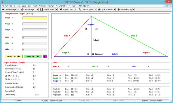
Figure 391 is the result with three sides. The triangle shown is the generic triangle with labels to assist in decoding the parts of the triangle. Use the [Esc]ape key to bring up the scale triangle.

Figure 392

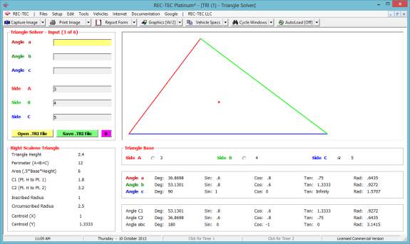
Figure 392 is the result with three sides. The dot in the triangle represents the centroid. The triangle shown is drawn to scale.

Figure 393

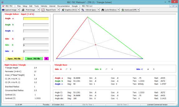
Figure 393 displays the lines proving the dot is the centroid. The lines are toggled by right clicking on the scale triangle.

Figure 394

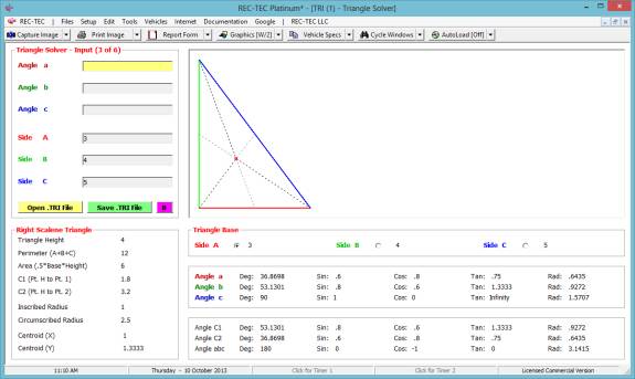
Figure 394 displays the scale triangle with Side A selected as the base.

Figure 395

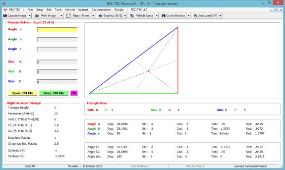
Figure 395 displays the scale triangle with Side B selected as the base.

Example 2: Angle a = 15, Side A = 3, and Side C = 5

What is the length of Side B?

Figure 396

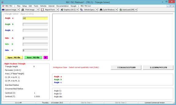
Side B could be either dimension. Select the first root. This is displayed in Figure 397

Figure 397

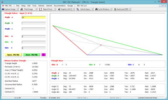
Example 3: Select the second root. This is displayed in Figure 398.

Figure 398

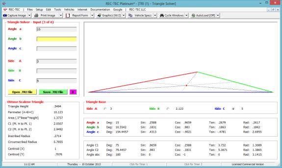
Example 4: Angle a = 60, Side B = 5, and Side C = 5

Figure 399

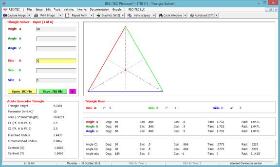
Module 45: Statistical Range (Monte Carlo)

(Table of Contents)

Overview: This module provides mathematical justification for the ranging of variables based on a limited number of samples.

At the REC-TEC pull down menu, select Statistical Range (Monte Carlo) and the Monte Carlo – Range screen appears (Figure 400).

Figure 400

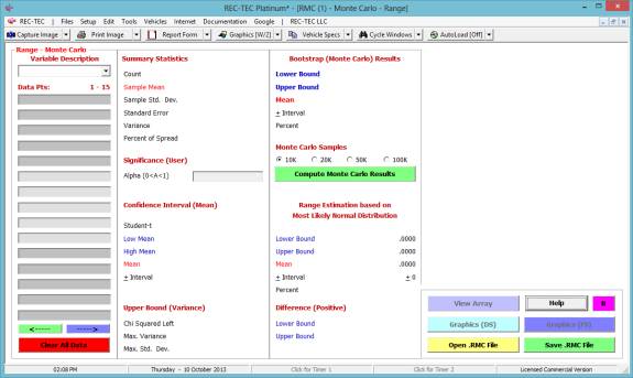
Required Input Data

· Optional (Name of variable being analyzed)

· Data points – The number of data points is limited by the amount of computer memory. The screen only shows 15 data points at a time.

A full description of the outputs, including a legend of the colors used for the various curves is contained in the F1 key – Help files.

This module will do a Statistical Analysis of the data points. If desired, it will also do a Monte Carlo Analysis of the data using 10K, 20K, 50K, or 100K samples. The samples are written to a file and may be printed if necessary. The greater the number of samples needing processing, the longer the time required. The program will indicate the progress of the processing.

This module is based on the following paper, which the author has graciously allowed REC-TEC to use as the Help file: Finding a Range Using Statistics In Traffic Crash Reconstruction by Jeremy Daily, Jackson Hole Scientific Investigations, Inc., 19th Annual Traffic Crash Reconstruction Conference, Illinois Association of Technical Accident Investigators (IATAI), September 20, 2005.

Example 1: Four separate runs to determine drag factor were made using an accelerometer. The results were 0.763, 0.72, 0.751 and 0.743.

Do a statistical analysis of these data points and include a Monte Carlo analysis using 100,000 samples.

Figure 401

Figure 401 shows the basic statistical data and the Monte Carlo analysis.

Figure 402

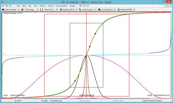
Figure 402 shows the composite view of all of the curves. Each curve consists of 100,000 points that are individually plotted. The four large red points are the entered data points on the Monte Carlo CDF curve.

Figure 403

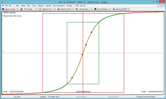
Figure 403 shows the Monte Carlo CDF curve.

Figure 404

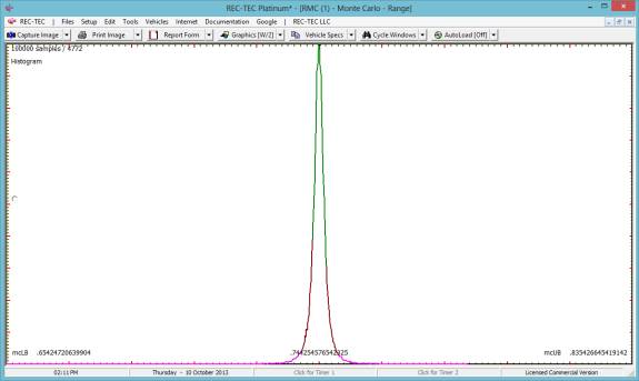
Figure 404 shows the Histogram curve.

Figure 405

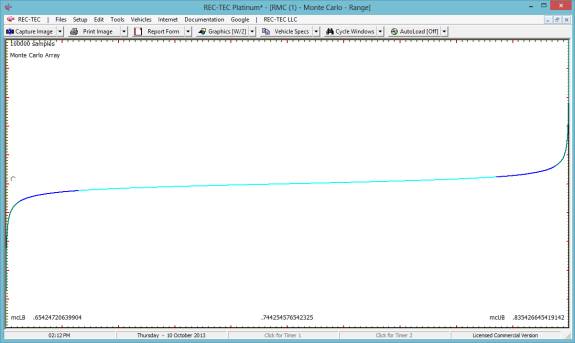
Figure 405 shows the Monte Carlo array curve.

Figure 406

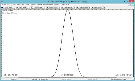
Figure 406 shows the Monte Carlo PDF curve.

Figure 407

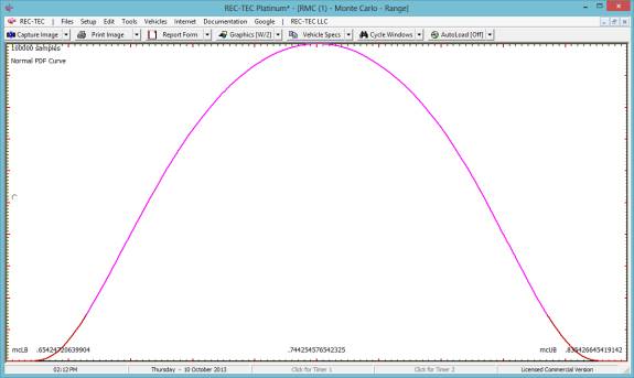
Figure 407 shows the Normal PDF curve.

Figure 408

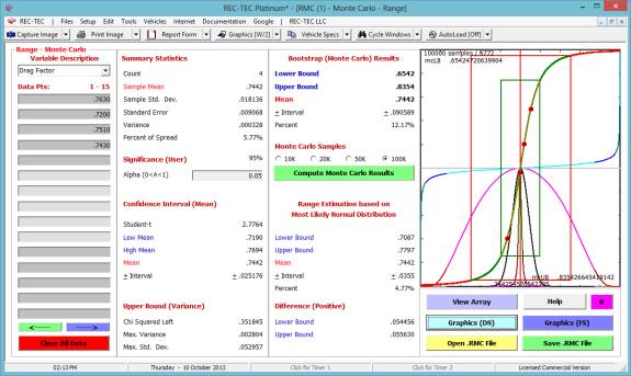
Figure 408 shows the composite of all curves along with the numerical data.

Figure 409 shows the data from Time - Distance Omni (Module 8), Example 3, Figure 104, but without the Monte Carlo run.

Figure 409

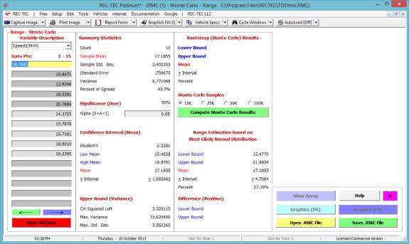
Figure 410

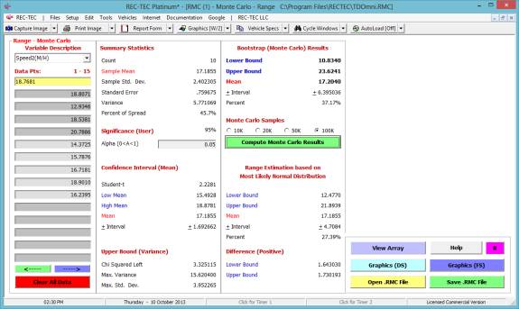
Figure 410 shows the numerical data including a 00K Monte Carlo run.

Figure 411

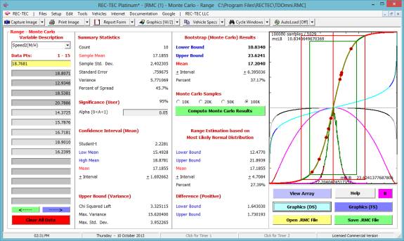
Figure 411 shows the numerical data including the new 100K Monte Carlo run and the composite of all curves drawn with a line width of 1.

Figure 412

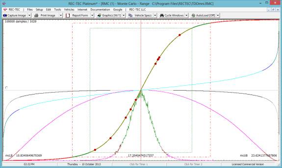
Figure 412 shows the full screen composite of all curves drawn with a line width of 1.

Module 46: Photogrammetry – REC-TEC 2D Photogrammetry

(Table of Contents)

Overview: This module provides two-dimensional numerical rectification of photographic images.

Before getting into the technical details of Photogrammetry, there are two basic questions that should be answered: 1) What is needed; and 2) How is it done?

Needed:

1. A photograph of an area containing something that we need to measure.

2. A scale diagram of the 2D (planar) questioned area of our photograph.

3. 4 points on the 2D area of the photograph, which also appear on the scale diagram and that surround the area where measurements are needed.

How it is done:

1. The X and Y coordinates of the 4 points from the photograph are entered into the appropriate entry blocks in the REC-TEC Photogrammetry module.

2. The X and Y coordinates of the 4 points from the scale diagram are entered into the appropriate entry blocks in the module.

3. With the photograph now numerically linked to the scale diagram (yes, that is already done), it is time to enter as many points from the photograph into the X and Y Photographic entry blocks, located below the Calibration section, as needed. There is also an optional entry block for Comments that can contain a description of the point that will be recorded in the printable Table being built.

Note: The diagram X and Y coordinates are best measured directly from the scale diagram. There are choices when measuring the X and Y points from the photograph:

· If an electronic image is loaded into the Photogrammetry module, the cursor can be activated allowing the Mouse to transfer both the X and Y points of the cursor position directly to the input blocks for the Photograph point. The program will convert these points to Scale Diagram points, displaying both in the appropriate blocks ready for transfer to the Table and the Image. This fast and easy and will all be discussed later.

· A scale grid can be superimposed over the photograph. The scale need not be the same as the diagram. It must allow assigning X and Y coordinates to positions of interest on the photograph for manual entry into the program.

· An electronic image can be taken of the photograph and loaded into the module as described above.

General: This module will allow the user to take accurate measurements from a photograph. If the user can match four (4) points on a photograph with the corresponding points on a scale diagram, then any points that are in the same physical plane as the calibration points can be placed in the correct position on the scale diagram. The diagram need not be in the same scale as the photograph. The camera, lens (except fisheye and extreme wide angle lenses), and position from which the photograph was taken, are not of overriding importance. There must be four (4) points in the same plane on the photograph that are also on the scale diagram. The solution points must be in the same plane. No more than two (2) of the points can be in the same straight line. A grid, divided into coordinates, must be superimposed over the photograph. The scale diagram must be divided into coordinates, but not necessarily to the same scale as the photograph. Each different photograph must be done individually. The calibration is for one photograph only.

Each of the four (4) calibration points on the photograph is linked to its corresponding position on the scale diagram. The photograph is numerically calibrated to the scale diagram. Once this is accomplished, any point on the photograph within the area surrounded by the calibration points will generate a corresponding point on the scale diagram – simple, easy, quick, efficient, and very accurate.

2D PHOTOGRAMMETRY

Calibration Points:

Photograph 1 (X) Photograph 1 (Y)

There is no default. Place the X and Y co-ordinate of the first point on the photograph.

Scale Diagram 1 (X) Scale Diagram 1 (Y)

There is no default. Place the X and Y co-ordinate of the first point on the diagram.

Repeat this procedure for points two (2) through four (4).

Calibration Factors:

These factors are the answers to the matrix. They are used to solve for the points that will be fed into the program.

NOTE: The program checks the slope of the line between points in an attempt to prevent three (3) points in the same straight line from being entered. The program may not allow solutions for legitimate points depending on how the points are entered due to this check. This problem can be overcome by entering the points in a different order.

If the following points are entered, then the program will reject an attempt at a solution.

Photograph: 1,1 2,1 2,2 1,2 Scale Diagram: 1,1 2,1 2,2 1,2

The rejection is based on the fact that the slope between points 1 & 2, and points 3 & 4 is the same (0). These points should be entered as:

Photograph: 1,1 2,2 2,1 1,2 Scale Diagram: 1,1 2,2 2,1 1,2

By changing the order in which points are entered the program will accept the points for solving the matrix.

Solution:

Photograph N (X and Y)

Enter the coordinates of the points on the Photograph.

Photograph N (X) = N.NNNN Photograph N (Y) = N.NNNN

These are the X and Y coordinates of point (N) on the photograph.

Scale Diagram N (X) = N.NNNN Scale Diagram N (Y) = N.NNNN

These are the Computed X and Y coordinates of the corresponding point (N) on the Scale Diagram.

No Solution:

No solution for the points given. Usually the points were entered incorrectly, or three (3) of the points are in a straight line.

At the REC-TEC pull down menu, select Photogrammetry > REC-TEC 2D Photogrammetry and the Photogrammetry screen appears (Figure 413).

Figure 413

Required Input Data

Calibration Points (1-4)

· Photograph (1-4): – X and Y Coordinates for Photograph Points (1-4)

· Scale Diagram (1-4): – X and Y Coordinates for Scale Diagram Points (1-4)

· Computed Point (1-4): – Program “check solves” for Scale Diagram Points (1-4) above.

Solution Points (N)

· Enter: Photograph (N): – X and Y Coordinates for Photograph Point (N)

· Computed: Scale Diagram (N): – X and Y Coordinates for computed Scale Diagram Point (N)

IPTM Publications – The following publications available from IPTM 1-904-620-4786 or http://www.iptm.org and are recommended for further reading:

· ANATOMY of a COLLISION by George M. Bonnett includes the below listed article.

· BASIC PHOTOGRAMMETRY by George M. Bonnett contains an article discussing basic 2-Dimensional Photogrammetry using Numerical Rectification.

Example 1: This first example is really a calibration check that will verify that the module is functioning correctly. After the calibration, the input numbers should match perfectly with the “solution” numbers. There will be only two examples, as using Photogrammetry correctly will take more study and a lot of practice.

Figure 414

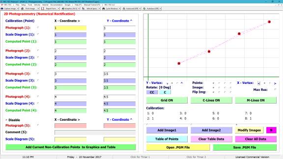
Figure 414 shows the graphics for the calibration entries.

Figure 415

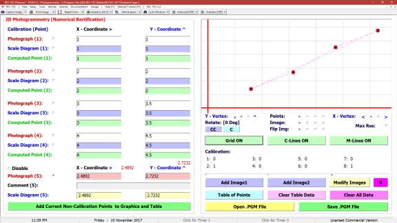
Figure 415 shows the solution/verification entries.

Figure 416

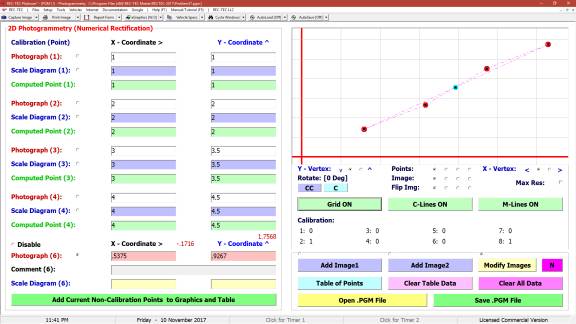
Figure 416 shows the graphics of the calibration and solution/verification entries after clicking on the “Add Current Non-Calibration Points to Graphics and Table” button.

Figure 417

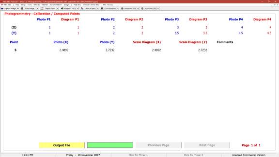
Figure 417 shows the table of calibration and solution/verification entries on the Table of Points.

Figure 418

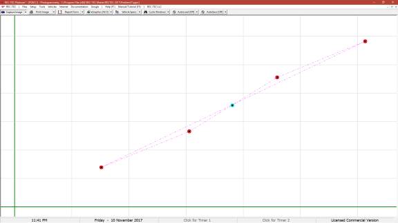
Figure 418 shows the full-screen graphics of the calibration and solution/verification entries.

Figure 419

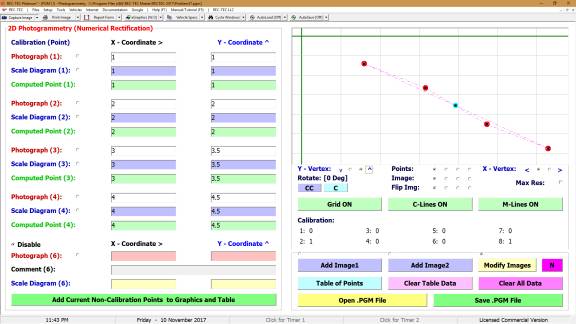
Figure 419 shows the graphics of the calibration and solution/verification entries with the Y-vertex inverted using the radio button at the left just below the graphics.

Example 2: This is a problem from the Basic Photogrammetry article.

Figure 420

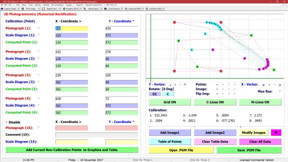
Figure 420 shows the graphics of the calibration and solution entries.

Figure 421

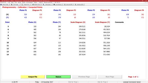
Figure 421 shows the table with calibration and solution entries.

Now for some of the new features, notice that on the left hand side of the screen there are Radio Buttons next to all of the Photograph points, and next to the Scale Diagram points after the 4 Calibration points. There is also a Disable radio button defaulting to ON. Selecting any of these radio buttons except the one for Disable turns Mouse tracking ON when the Cursor is over the Graphics screens. The X and Y positions are shown near the X and Y - Coordinate labels on the small graphics screen and in the upper-left corner of the large graphics screen. Clicking the Right Button on your Mouse transfers the X and Y coordinate positions of the cursor to the input boxes for the Photograph/Scale Diagram selected by using the radio buttons. This automatically calculates the Scale Diagram points.

The X and Y Axes are normally Green with line width determined by eGraphics when Mouse Tracking is not active. When Mouse Tracking is active the Axes turn Red with a line width of 5 to remind the user that the right mouse button is hot.

Figure 421A

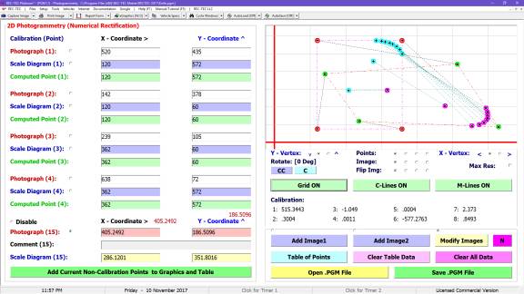
Figure 421A shows the coordinates in red and the data transferred to the Photograph X and Y inputs.

Figure 421B

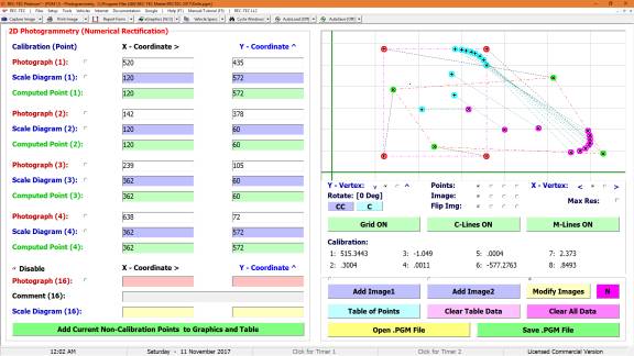
Figure 421B has the data transferred to the Table and shown on the graphics screen as both a Photo point and a Scale Diagram point.

Figure 421C

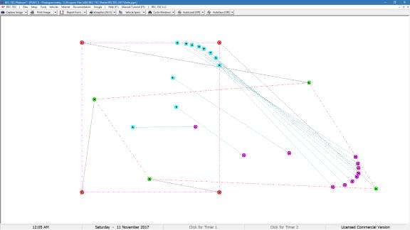
Figure 421C has the Grid turned to Off.

There are two more new features in the revised module. The “Add Image1” and “Add Image2” buttons may not have escaped notice, but the 3 tiny radio buttons above them may have. ToolTips will give the secret away, it they are activated by the cursor.

Add Image1 and Add Image2 will each add and save an image in memory. The radio buttons control which of these images will be displayed. The third radio button removes the images from the display screens. They can be replaced by pressing one of the other radio buttons. To permanently an Image, click the “Image(N) On” button and when the Dialog Screen appears, click on Cancel.

Figure 421D

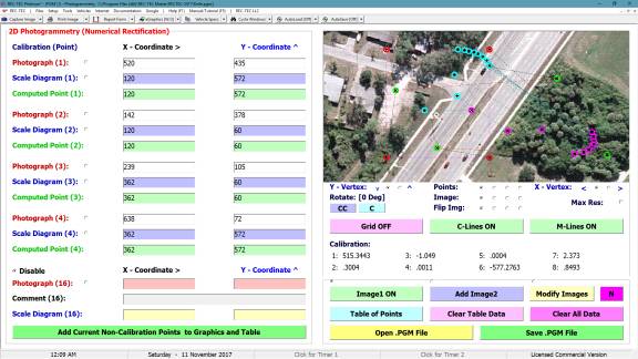
Near the center of the right panel are 3 labels, Image, Display and Flip Img. Each label has 4 radio buttons.

Display determines which Points are displayed - All Points, Photographic Points, Scale Diagram (Map or Overhead Image), or No Points.

Image controls how the background Image (if any) is scaled to the Picturebox - Width, Width > Height, Width < Height, or Height. (Read “>” as “greater weight than” and “<” as “less weight than.” See Figure 421E which shows the new Image controls.

Flip Img manages the Background Image - No Flip, Flip Vertical, Flip Horizontal, or Flip Vertical and Horizontal.

In the rare instance that it is necessary to Rotate (change the orientation) of the Images, Microsoft Paint can perform this task easily, and it can modify the images in some very intriguing ways, such as placing two images (Photo and Diagram) side by side on the same image.

Note: Unless it is strictly for “practice”, using an Image2 Diagram is probably not a good idea, as then this diagram should really calibrated to your Scale Diagram. If using an overhead ophthalmic mosaic as the diagram, it should give good approximate positions, but stick with the same (small or full screen view) as the change of aspect ratio does alter the position slightly as can be seen below.

Figure 421E

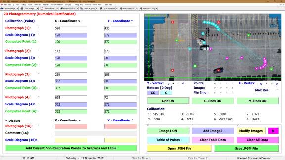
Figure 421F

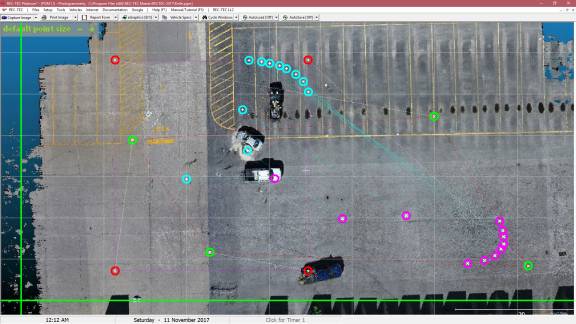
Figure 421F has the circles on the points set to 5 using the eGraphics dropdown menu.

The image shown is not related to the coordinate positions shown. Images can be used to show both a Scale Diagram and the Photograph containing the Control Points and the other points to be transferred to the Scale Diagram. The ability to use the mouse to set the Control Points and then to select the questioned points to be transferred makes for a quick and efficient process that eliminates transfer errors that could arise when using manual entry of the points.

The questioned points and the calibration points must all be located on the same plane. While a two-dimensional plane is a prerequisite, this plane need not be a horizontal surface. There is also no requirement that the entire photograph be of a single planar surface, only the area being examined must be planar.

Once all of the points in the same plane on the photograph have been identified on the actual scale diagram, accurate measurements can then be taken from the scale diagram.

Module 47: Heavy Truck – DISC/S-CAM III/V Air Brake

(Table of Contents)

Overview: This module computes and simulates the deceleration of S-CAM or Air Disc equipped vehicles based on Initial Speed or Distance and the setup and adjustments of the vehicles braking system. This module compensates for the heat created during the run. In Enhanced ABS mode the instantaneous Chamber air pressure differential set by the user is maintained throughout the course of the run. This advanced feature is only available in REC-TEC Platinum.

The new generation V module accommodates the use of a different surface friction on the left and on the right side of the vehicle. If both sides have the same friction value, it will do Finite Difference Analysis based on the single friction value. If the sides have different values it does an independent analysis on each side to reach an uncertainty value.

There is also a check block for a Single Air Control Modulator that would use the air pressure on the locking wheel for both chambers. A second check box is available in the event the Modulator is cross-wired and is using the higher air pressure of the non-locking wheel.

The generation V module is capable of changing many of the initial inputs during the course of the run including the left and right side surface frictions, grade, air pressure, and sensor condition using a distance domain matrix. This capability allows the simulation of acceleration, deceleration and constant velocity at varying distances during the run.

At the REC-TEC pull down menu, select Heavy Truck > DISC/S-CAM III/V Air Brake and the DISC/S-CAM III/V Air Brake screen appears (Figure 422).

Figure 422

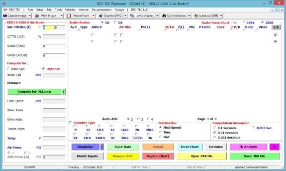
Required Input Data

· Surface Friction – Measured

· C/TTD – Car Truck Tire Differential – adjustment to Surface Friction

· Grade (Test) – Grade at Friction Test Area – used to correct to level if Surface Friction not measured at Actual site

· Grade (Actual) – Grade at Area under scrutiny (Scene)

Compute for: (Button)

· Initial Speed – Solves for Initial Speed using input value for Distance (Iteration)

· Distance – Solves for Distance using input value for Initial Speed

Compute for Distance/Initial Speed: (Command Button to initiate computations)

· Final Speed – Final Speed of Vehicle in this run (multiple runs possible)

· Steer Axles – Number of Steer Axles

· Drive Axles – Number of Drive Axles

· Trailer Axles – Number of Trailer Axles

· Temp – Temperature of brakes at Start of (first) run (See Temperature note infra)

· Air Press (M) – Master Air Pressure/Percent - This value multiplied by Psi(E) value equals Chamber Pressure. User may elect to use 100(%) here and use actual Chamber Air Pressure for individual Wheels

Brake Status

· CS (Cold Stroke) – Changes Display to show Cold Stroke Pushrod Force

· DS (Dynamic Stroke) – Changes Display to include Initial Dynamic Increment to Cold Stroke and the Heat Increment at the Start Temperature

Brake Force Chart

· 1991 – Uses original charts with minor upgrades for newer chambers

· 2008 – Uses completely updated charts including new manufacturer’s specifications (created in collaboration with Ron Heusser, and Wesley Grimes)

The following information list pertains to each axle end in the configuration:

A/S – Axle Number / Side (Left/Right)

· Type – Chamber Type – Enter directly or select from Chamber Type (below)

· ABS Checkbox – Check for ABS brake

· ABS % – Enter ABS% of Conventional Brake based on type/Cyclic rate

· Air Disc Checkbox – Check for Air Disc brake

Lift – Enter horizontal distance the power shaft travels in one complete revolution for Air Disc if not default

· Psi(E) – Psi(E) Chamber Pressure/Percent - This value multiplied by Master Air Pressure/Percent value equals Chamber Pressure. Enter as Percent (%) or Actual Pressure at Chamber. Dependent on entry for Air Press – this is opposite of Air Press entry. Entering a zero (0) or blanking out the entry turns the brake inoperable and it becomes freewheeling unless it is locked.

· Slk L – Length of Slack Adjuster (measured)

· f(L) – Friction value of Brake Pad

· PRc – Pushrod Stroke (Cold - measured)

P Force – Shows either the Cold Stroke Force or the Stroke incremented for the Initial Dynamic Increment adjusted for Start Temperature. (User Selectable)

· Lock(<) – Minimum Force required to Lock Brake for Load

· r-P/D – (Air Disc) distance from Center of Pad to Wheel Axis / Drum Radius

· R-rad – Rolling Radius of Wheel (measured Center to Surface)

· Vload – Vertical Load on Axle end

· Lck – Checkbox to Lock Wheel regardless of data entered

Termination – Selection allows termination of run for multiple (Segmented by Time or Distance or Speed) runs or at Collision Speed as required.

· Final Speed

· Time

· Distance

Computation Increment – Sets the Time increment between computations during run. Accuracy increases as increment is shortened between “looks” at the status of all of the brakes in the system.

· 0.1 Seconds

· 0.01 Seconds

· 0.001 Seconds

· 0.033 Seconds (Animation output)

Example 1: This example uses the file Problem44.trk as the basic problem. It will be used to show the different capabilities of the module.

Figure 423

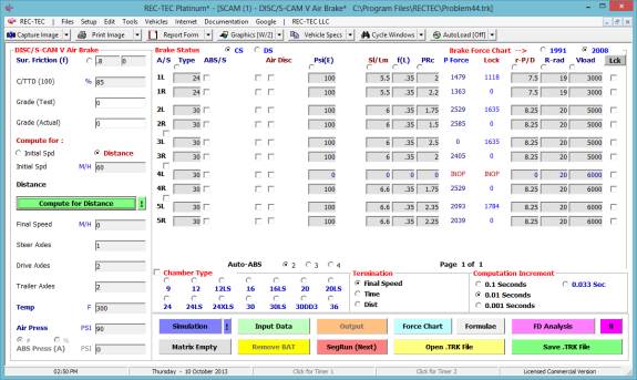
Figure 423 displays the screen exactly as it appears after the file is loaded. Computation is for Distance with a given Initial Speed of 60 M/H.

Figure 424

Figure 423 displays the screen after clicking on Compute for Distance. Both input and computed data are displayed as well as the final status of each brake. The legend for the screen is in the F1key – Help file.

Figure 425

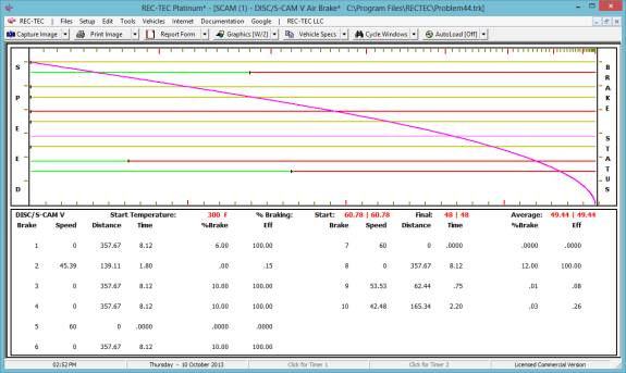
Figure 425 displays the Simulation screen. The upper portion consists of a line showing at which point the brake changes status from Operational to Failed. The lower portion displays counters (paused and resumed with the Spacebar) that lock when the brake fails.

Figure 426

Figure 426 displays the Finite Difference Analysis menu. The range for the variables is shown in the menu.

Figure 427

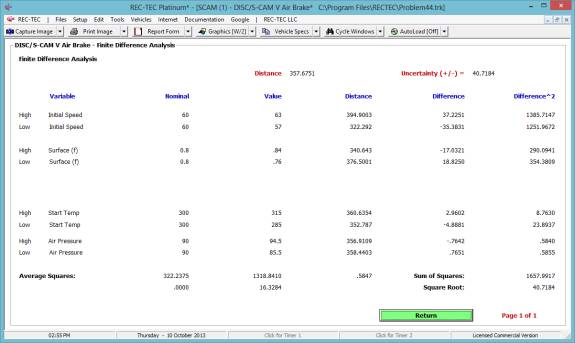
Figure 427 displays the Finite Difference Analysis and the resulting uncertainty of the distance.

Example 2: Using the file Problem44.trk as the basic problem, solve for Initial Speed using a distance of 400 feet.

Figure 428

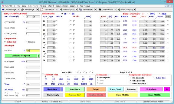
Figure 428 displays the screen when the Computation is set for Speed using a given Distance of 400 feet. This is the one change made to the file as initially loaded.

Figure 429

Figure 429 displays the screen after clicking on Compute for Distance. Both input and computed data are displayed as well as the final status of each brake. The legend for the screen is in the F1key – Help file.

Figure 430

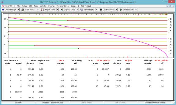
Figure 430 displays the Simulation screen. The upper portion consists of a line showing at which point the brake changes status from Operational to Failed. The lower portion displays counters (paused and resumed with the Spacebar) that lock when the brake fails.

Figure 431

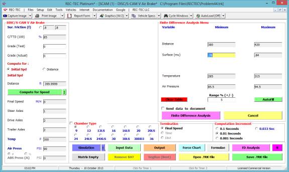
Figure 431 displays the Finite Difference Analysis menu. The range for the variables is shown in the menu.

Figure 432

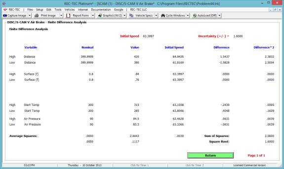
Figure 432 displays the Finite Difference Analysis and the resulting uncertainty of the Initial Speed.

Example 3: Using the basic information from example 1, make the following changes:

· 1L and 1R MaxP @ 80 and check Air Disc (2.125 & 7.5)

· Lock (checkbox) wheel 4R

· Set Grade (Actual) at –0.05

· Set Final Speed to 30 M/H

· Check Enhanced ABS Computations & set ABS Pressure to # 5

Figure 433

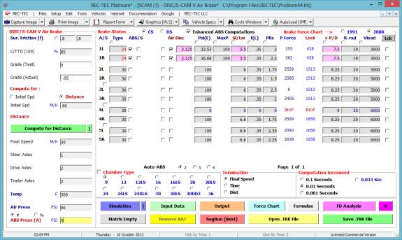
Figure 434

Note: Acceleration due to gravity exceeds brake force (negative number) for some wheels.

Figure 435

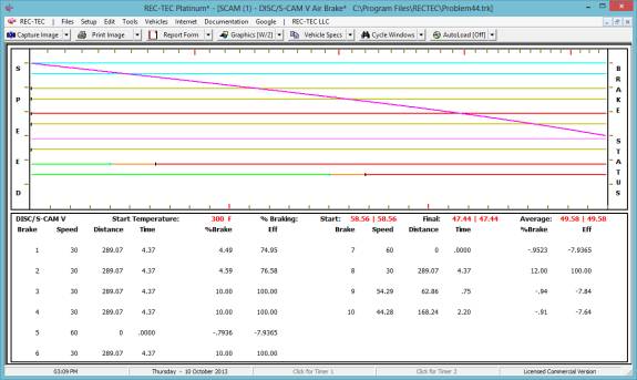
Figure 435 shows the transition areas (bottom two axles) where acceleration due to gravity exceeded braking. Notice that the Deceleration curve goes from 60 M/H to 30 M/H.

Figure 436

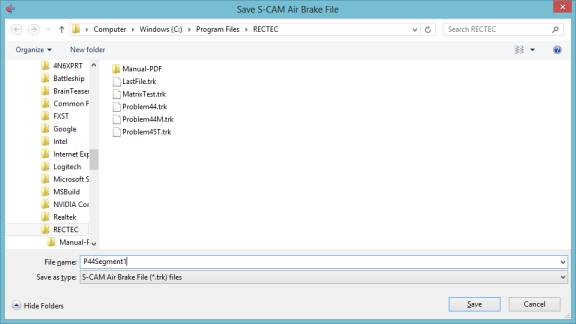
Figure 436 urges saving the current segment as a named file after clicking “Segmented Run” on the screen shown in Figure 433. After saving this filename, the program automatically makes the transition to the screen shown in Figure 437. This includes transferring the current Brake Activation Time (BAT) forward for correct computation of the heat build-up during the course of additional segments.

Figure 437

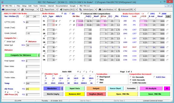
Figure 437 shows the second phase of the segmented run. Change the Air Pressure (Screen left-bottom) to 65 pounds and the Surface Friction to 0.65.

Figure 438

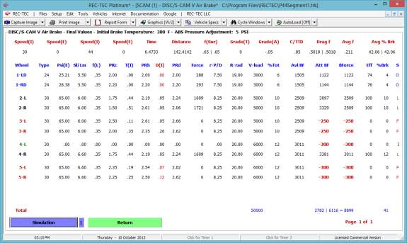
Figure 438 displays the screen after clicking on Compute for Distance. Both input and computed data are displayed as well as the final status of each brake.

Figure 439

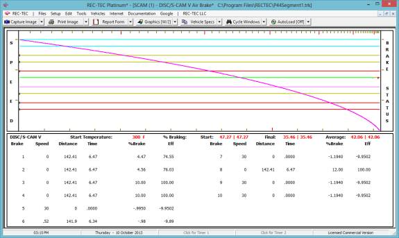
Figure 439 shows the transition areas (wheels 5, 7, and 8) where acceleration due to gravity exceeded braking. Notice that the Deceleration curve goes from 30 M/H to zero (0) M/H.

This completes the second phase of the segmented run. The runs can be broken up by time, distance, or speed into as many segments as desired. The transition is accomplished automatically except for naming the file to be saved. This will assist where different surfaces are encountered, air pressure drops for some reason including depletion resulting from the cycling of an ABS system, or any other circumstance requiring a mid-run change to the initial data.

Example 4: Using the basic information from example 1, make the following changes:

· Change the Start Temperature to 450 degrees.

What is the distance to stop?

Example 5: Using the basic information from example 1, make the following changes:

· Change the Start Temperature to 650 degrees.

What is the distance to stop?

Example 6: Using the basic information from example 1, make the following changes:

· Change the Start Temperature to 850 degrees.

What is the distance to stop?

S-CAM V Matrix (Platinum only) permits almost all of the segmented run changes to be computed and displayed in a single “Run” as opposed to the “Segmented Run” computations.

Figure 439-M1

Figure 439-M2

Figure 439-M3

Figure 439-M4

Matrix Inputs – Calls up a distance-domain based matrix allowing 15 separate interrupts during the simulation for changing the Surface Friction, Grade (Actual), Pressure (A), disabling the individual brakes by zeroing the air pressure in any chamber as well as disabling any of the individual ABS sensors. Setting the friction (and grade) to zero, allowing the vehicle to maintain a constant velocity. A negative value for friction (or grade) will accelerate the vehicle. In addition the user can now lock any of the brakes or can engage the Spring Brake at a selected wheel. Engaging a Spring Brake allows the user to set the Equivalent Air Pressure for the individual Spring Brake (usually the air pressure required to disengage the Spring Brake). These capabilities will allow the simulation to mimic most three-dimensional trajectories. Placing the cursor on the Wheel Designation next to a disabled checkbox for a particular mode will give information on the Interrupt Distance and, in the case of a Spring Brake, will display the Equivalent Air Pressure.

Matrix Maneuvers – The Matrix provides the user with the ability to “coast” with either a user selectable deceleration, or with no deceleration by modifying the drag factor (Mu) value at any distance interrupt during the run. Using a Mu value greater than zero (0) will cause the vehicle to decelerate provided at least one of the brakes is decelerating enough to overcome any downhill grade. A zero (0) value will cause speed changes dependent on grade only.

The Matrix will also allow any activated Spring Brakes to control the deceleration of the vehicle if no other braking is engaged. In order to set this up, the Mu should be set to the proper value and at least one of the Spring Brakes must be engaged. The user may then select an Air Pressure [Air(P)] value of zero (0) at the appropriate interrupt. Multiple interrupts may be set to zero (0) with changes made to different settings at the different interrupt points to simulate the conditions of the maneuver in question. The user is advised to meticulously check all changes to insure that they are not antagonistic or self-canceling. The program uses an elaborate hierarchy to prioritize the settings. Care should be exercised to insure that the answers generated are consistent with what could be reasonably expected to occur during the maneuver. Exotic/multiple failures should be given wide ranges absent collateral proof of the accuracy of the computations.

Matrix Color Legend – Left side wheels are Green and Right side wheels are Red. Wheels color-coded Blue are modified in the Matrix for the particular Mode (PSI, Sen, Lock, or S-Brk) selected by the User. Wheels color-coded Black are set that way on the main interface.

Color Legend:

Yellow = Locked

Purple = Spring Brake only

Green = Operable – not locked

Red = Failed

Orange = Braking not able to overcome grade

Pink = Inoperable

Dark Blue = ABS Air Disk (sensor)

Light Blue = ABS Air Disc (no sensor or slaved)

Dark Gray = ABS S-Cam (sensor)

Light Gray = ABS S-Cam (no sensor or slaved)

Figures 439-M5 through 439-M8 show a ramping up of Air Pressure as the Brakes are first applied. This ramp-up of Air Pressure in the chambers takes just over a half a second as it reaches 90 pounds in 50 feet with a start speed of 60 M/H.

Note: These numbers are fictitious and do not represent the values that may be encountered in any given situation. They are used for illustrative purposes only.

Figure 439-M5

The file shown in Figure 439-M5 is identical to Problem44.TRK except that the starting Air Pressure is set to 1 and there is an Active Matrix. (Note: The program will not function with an Air Pressure of Zero (0).

Figure 439-M6

Figure 439-M6 shows the values set into the Matrix.

Figure 439-M7

Figure 439-M7 shows the final data values for the run.

Figure 439-M8

Figure 439-M8 shows the animation solution for the run.

Figure 439-M9

Figure 439-M9 shows the animation solution for the run for Problem44.TRK.

Module 48: Heavy Truck – Load Check A (Tractor - Trailer)

(Table of Contents)

Overview: This module computes Articulated Vehicle axle weights and three-dimensional center of gravity based on information about vehicle and load (Bill of Lading).

At the REC-TEC pull down menu, select Heavy Truck > Load Check A (Tractor - Trailer) and the Load Check A (Tractor - Trailer) screen appears (Figure 440).

Figure 440

Required Input Data – Tractor

· Wheelbase: – Wheelbase of Tractor

· Front-SA: – Distance from the Front of the Vehicle to the Steer Axle

· 5W-cDA: – Distance from the Fifth Wheel to the Centerline of the Drive Axle(s)

· Drive Axles: – Number of Drive Axles

· Tire Radius: – Distance from the Center of the Axle to the Road Surface

· TR CG (Lng): – Distance (Longitudinal) from the Front to the CG (Tractor)

· TR CG (Ver): – Distance (Vertical) from the Road Surface to the CG (Tractor)

· TR Weight: – Weight of the Tractor

Required Input Data – Trailer

· Length: – Overall Length of Trailer

· Height: – Overall Height of Trailer

· Width: – Overall Width of Trailer

· TL (hBed): – Bed Height of Trailer

· TL CG (Lng): – Distance (Longitudinal) from the Front to the CG (Trailer)

· TL CG (Ver): – Distance (Vertical) from the Road Surface to the CG (Trailer)

· TL Weight: – Weight of the Trailer without Load

· Front-KP: – Distance from the Front of the Trailer to the Kingpin

· KP - cRA: – Distance from the Kingpin to the Centerline of the Trailer Axle(s)

· TL Axles: – Number of Trailer Axles

· Tire Radius: – Distance from the Center of the Axle to the Road Surface

Required Input Data – Load – Note: When inputting the Load information:

1. Disregard the Total number of Loads in Loads (#) – it should be 1 at the start. To delete all loads, enter a Zero (0) for Total number of Loads

2. If necessary, Click the Right (or Left) Arrow button at Current (#) to bring up the (next) appropriate Load number in the Current Load box (Start with Load # 1)

3.  After entering all of the data for the Load, click on the DO button

4.  Go to Step 2 until you have entered information for all of the Loads

5.  If the Graphics are not displayed, Click on Graphics.

· Loads (#): – Number of Individual Loads

· Current (#): – Number of Current Load (Enter or use Arrows to Change)

· Height (Ver): – Vertical Height of Current Load

· Length (Lng): – Longitudinal Length of Current Load

· Depth (Lat): – Lateral Depth of Current Load

· Weight: – Weight of Current Load

Required Input Data – CG Location of Current Load

· CG% (Btm): – Location of CG from Bottom of Current Load

· CG% (Frt): – Location of CG from Front of Current Load

· CG% (Lft): – Location of CG from Left Side of Current Load

Required Input Data – Position of Current Load

· Lng (X): – Longitudinal Distance: Front of Trailer to Front of Current Load

· Lat (Y): – Lateral Distance: Left of Trailer to Left of Current Load

Example 1: The input data is shown on Figure 441 including the load information for Load #1, which is the only load.

Figure 441

Notice that in Figure 441 there is an Adjustment button. This button will toggle (on/off) four different slider-bars allowing adjustments to the Graphics screen. The small slider-bar under the Adjustment button controls the size of the tractor and trailer. The slider-bar on the left side of the screen controls the vertical position of the overhead view. The slider-bar on the right side of the screen controls the vertical position of the side view. The slider-bar on the bottom of the screen controls the horizontal position of both the overhead and side view. The Checkbox above the Graphics button will draw CG markers for the Tractor (Blue), the Trailer (Red), the Load (Green), and the entire unit (Black). See Figure 442.

Figure 442

Figure 443

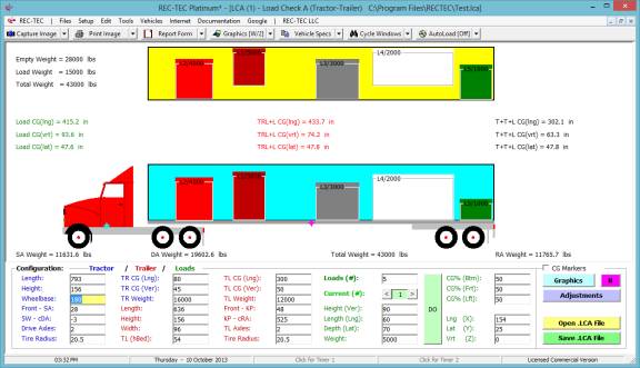
Figure 443 shows a Tractor-Trailer with five different loads. The individual loads may be shifted using drag-drop, or positioned using the text boxes for load positioning. In addition, the fifth-wheel may be repositioned in the same manner. A maximum of 1-steer axles, 5-drive axles and 5-trailer axles are permissible.

Module 49: Heavy Truck – Load Check B (Straight Truck - Bus)

(Table of Contents)

Overview: This module computes Straight Truck, Bus or other non-articulated Vehicle axle weights and three-dimensional center of gravity based on information about vehicle and load (Bill of Lading or passenger manifest).

At the REC-TEC pull down menu, select Heavy Truck > Load Check B (Straight Truck - Bus) and the Load Check B (Straight Truck - Bus) screen appears (Figure 444).

Figure 444

Required Input Data

Truck/Bus

· Wheelbase: – Wheelbase of Truck/Bus

· Front-SA: – Distance from the Front of the Vehicle to the Steer Axle

· Front-cBx: – Distance from the Front of Vehicle to the Front of Cargo Box

· Drive Axles: – Number of Drive Axles

· Tire Radius: – Distance from the Center of the Axle to the Road Surface

· Trk CG (Lng): – Distance (Longitudinal) from the Front to the CG (Truck/Bus)

· Trk CG (Ver): – Distance (Vertical) from the Road Surface to the CG (Truck/Bus)

· Trk Weight: – Weight of the Empty Truck/Bus

Cargo Box

· Length-cBx: – Overall Length of Truck/Bus

· Height-cBx: – Overall Height of Truck/Bus

· Width-cBx: – Overall Width of Truck/Bus

· Trk (hBed): – Bed Height of Truck/Bus

Load – Note: When inputting the Load information:

1. Disregard the Total number of Loads in Loads (#) – it should be 1 at the start. To delete all loads, enter a Zero (0) for Total number of Loads

2. If necessary, Click the Right (or Left) Arrow button at Current (#) to bring up the (next) appropriate Load number in the Current Load box (Start with Load # 1)

3.  After entering all of the data for the Load, click on the DO button

4.  Go to Step 2 until you have entered information for all of the Loads

5.  If the Graphics are not displayed, Click on Graphics.

· Loads (#): – Number of Individual Loads

· Current (#): – Number of Current Load (Enter or use Arrows to Change)

· Height (Ver): – Vertical Height of Current Load

· Length (Lng): – Longitudinal Length of Current Load

· Depth (Lat): – Lateral Depth of Current Load

· Weight: – Weight of Current Load

CG Location of Current Load

· CG% (Btm): – Location of CG from Bottom of Current Load

· CG% (Frt): – Location of CG from Front of Current Load

· CG% (Lft): – Location of CG from Left Side of Current Load

Position of Current Load

· Lng (X): – Longitudinal Distance: Front of Truck/Bus to Front of Current Load

· Lat (Y): – Lateral Distance: Left of Truck/Bus to Left of Current Load

· Vrt (Z): – Vertical Distance: Bottom of Truck/Bus to Bottom of Current Load

Example 1: The input data is shown on Figure 445 including the load information for Loads #1 and #2, which are the only loads.

Figure 445

Notice that in Figure 445 there is an Adjustment button. This button will toggle (on/off) four different slider-bars allowing adjustments to the Graphics screen. The small slider-bar under the Adjustment button controls the size of the Truck-Bus. The slider-bar on the left side of the screen controls the vertical position of the overhead view. The slider-bar on the right side of the screen controls the vertical position of the side view. The slider-bar on the bottom of the screen controls the horizontal position of both the overhead and side view. The Checkbox above the Graphics button will draw CG markers for the Load (Black) and the entire unit (Green). See Figure 446.

Figure 446

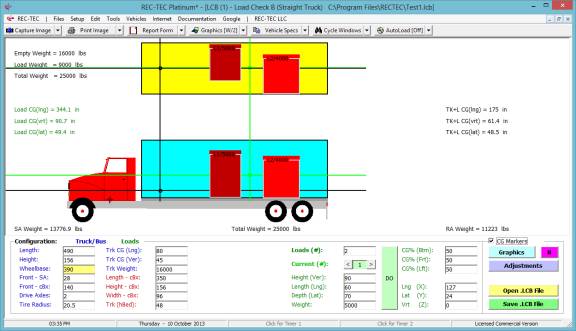
Figure 447

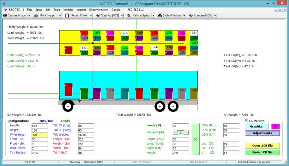
Figure 447 shows a School Bus with 38 different loads. The individual loads may be shifted using drag-drop, or positioned using the text boxes for load positioning. A maximum of 1-steer axles and 5-rear axles are permissible.

Module 50: Heavy Truck – Maximum Off-Tracking

(Table of Contents)

Overview: This module computes the Maximum Off-Tracking of articulated vehicles.

At the REC-TEC pull down menu, select Heavy Truck > Maximum Off-Tracking and the Maximum Off-Tracking screen appears (Figure 448).

Figure 448

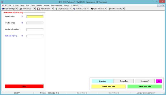
Required Input Data

· Steer Radius – Vehicle Steer Radius

· Tractor (WB) – Tractor Wheelbase

· Number of Trailers – Number of Trailers (0 to 3)

· Distance 0 (+/-) – Distance from the rear axle of Tractor (Towing Vehicle) to Articulated Point #1. Negative number indicates Articulated Point is forward of Drive Axle

· Trailer 1 (WB) – Trailer #1 Wheelbase (Kingpin to Center of Trailer Wheels)

· Distance 1 – Distance from the rear axle of Trailer #1 to Articulated Point #2

· Dolly 1 (WB) – Wheelbase of Dolly Converter #1

· Trailer 2 (WB) – Trailer #2 Wheelbase (Kingpin to Center of Trailer Wheels)

· Distance 2 – Distance from the rear axle of Trailer #1 to Articulated Point #3

· Dolly 2 (WB) - – Wheelbase of Dolly Converter #2

· Trailer 2 (WB) – Trailer #3 Wheelbase (Kingpin to Center of Trailer Wheels)

Example 1: A Tractor (18-foot wheelbase) with one Trailer with a length of 65 feet from the articulation point to the point measured for off-tracking (Wheels or rear of vehicle). The unit is turning with a steer radius of 250 feet. The articulation point of the vehicle is 1-foot in front of the drive axle.

What is the maximum off-tracking for this data?

Figure 449

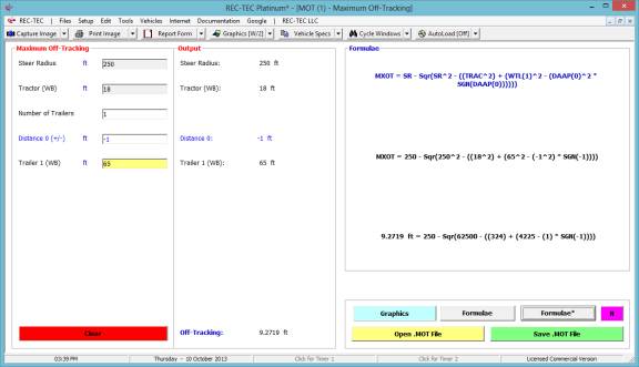
The maximum off-tracking is 9.2719 feet as shown in Figure 449.

Figure 450

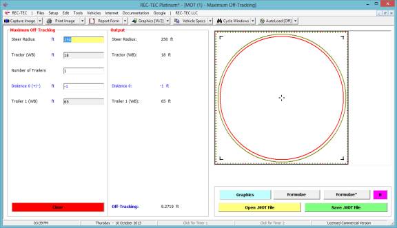
The Graphics for the maximum off-tracking event (9.2719) is displayed in Figure 450.

Example 2: Compute the off tracking of a "road train" with the following specs:

Wheelbase - tractor: 18 feet

Wheelbase - trailer #1: 48 feet

Distance - rear axle of #1 to articulated point #2: 2 feet

Weelbase - dolly converter #1: 4 feet

Wheelbase - trailer #2: 48 feet

Distance - rear axle of #2 to articulated point #3: 2 feet

Weelbase - dolly converter #2: 4 feet

Wheelbase - trailer #3: 48 feet

STEER RADIUS - 250 feet

Figure 451:

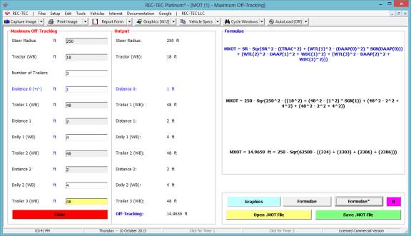
Example 3: Using the data from the above problem, what steer radius would you need to have a maximum off-tracking of 24-feet?

New Stuff added to Maximum Off-Tracking (April 2014)

Maximum Off-Tracking now has some new features. Using a zero (0) for the Steer Radius input will bring up a new series of inputs that will calculate the Steer Radius from either the Inner wheel Steer Angle or the Outer wheel Steer Angle. With Ackerman Steering, the two wheels will have different angles as they are turned from straight ahead.

The Graphics have also been modified (Platinum) to show the Vehicle in a scale turn based on the inputs. The next few pages will show the new additions to this module. It starts in entering a Zero for the Steer Radius at the top left of the Main Input screen, which brings up the Turn Radius Computation screen.

Figure 451B:

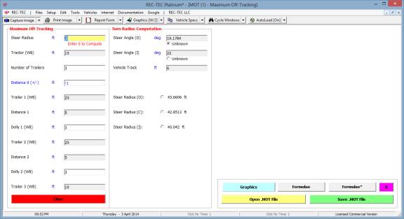
Entering 22 degrees for the Inner Steer Angle and marking the Outer Steer angle as Unknown calculates the Outer Steer Angle and the Steer Radii for Inner, Centerline, and Outer positions.

Figure 451C:

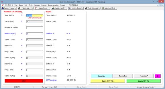
Selecting Formulae* in this configuration brings up Figure 451D.

Figure 451D:

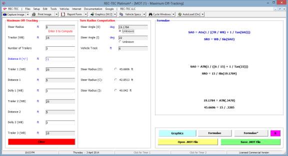
When a Steer Radius is Selected, that information is transferred and the Formulae* displayed will also change.

Figure 451E:

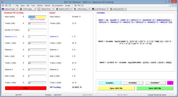
The initial Graphics selection still shows the twin circles in place of the Formulae* as seen in Figure 451F.

Figure 451F:

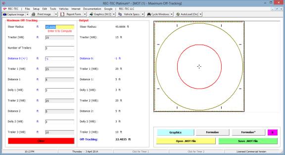
The display in Figure 451G is restricted to the Platinum version of the program.

Figure 451G:

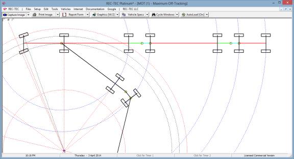
The figure across the top of the screen shows the vehicle as configured according to the inputs on the main input screen and includes the Vehicle Track on the secondary input screen. Note that the Rotation point of the vehicle is at the lower left of the screen resulting in part the vehicle configuration being drawn off of the screen.

In the upper left of the Screen there is a Checkbox and two Radio buttons. The Graphics can be manually set to show the Rotation point at either the 70% or 99% points on the screen or, when the drawing is off of the screen, right clicking on the mouse will automatically resize the drawing to the 70% position to allow the drawing to show the complete vehicle as in Figure 451H.

New Stuff added to Maximum Off-Tracking (Jan 2017)

The two Radio buttons have been moved to the primary Interface (Input) screen and defaulted to the 99% Rotation point. If this places part of the drawing off of the screen, right clicking on the graphics will automatically resize the drawing to the 70% position.

The checkbox to show Data on the Graphics screen has been enhanced to make it easier to find. There is also an input box allowing the user to input a Radius for radius-multiple (green) concentric circles to be drawn when the green Command button is clicked. The red Command button will draw a (red) Circle at the computed maximum off-tracking position.

Note: The “published“ formula will not compute the offset correctly if a trailer is beyond the 90-degree position relative to the straight-line (start) position. The Radius input allows the user to input a radius that will match the Maximum Off-Track. (Figure 451I)

New Stuff added to Maximum Off-Tracking (Feb 2017)

The algorithm used to display the vehicles introduced in January has been scrapped. Changing the frame of reference presented optimal coding resulting in a phenomenal increase in both speed and accuracy, so much so that the time to compute the solution and draw the vehicle is now shown in the upper right of the screen. The Graphics figures shown below reflect these new changes.

The increased speed allows changing the position of the 5^th wheel and the Steer Angle on the Graphics page with on the fly changes appearing almost instantly. Additionally both the 70% / 99% rotation points can be changed manually but are also integrated with the automatic selection for 70% on a redraw if required. Radius circles for each articulated unit are also displayed on alternate re-draws of the display (right mouse button). The new controls are shown below.

If the program encounters an error because the Radius is too small to accomplish the maneuver, it automatically resets to the last workable radius configuration. Using the smaller increment button will usually allow continued tightening of the turn.

Because the accuracy is so much better and the 90-degree restriction mentioned above has been totally eliminated, we are showing both the older “published” formula solutions along with the results of the new proprietary algorithm solutions on the Formulae* frame.

Figure 451H:

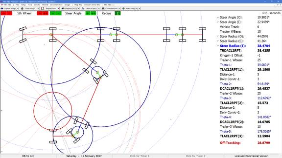
The Data portion of the screen has been expanded and is now permanent on the Graphics screen as seen in Figure 451H.

Figure 451I:

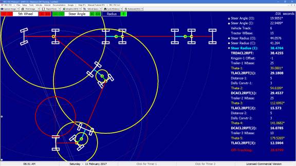
When returning to the Main input screen (Esc key) there will now be a Checkbox at the bottom of the Output panel. Checking this box will bring up Figure 451J showing the full Data Screen in the Output.

Figure 451J:

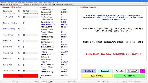
Note: Single Wheel sets are shown on all of the Graphics. Tandem or even Triple axles all rotate around the center of the axle set, therefore only single axles with single wheel sets are shown for the sake of simplicity.

Module 51: Heavy Truck – Rollover

(Table of Contents)

Overview: This module computes the Rollover Speeds of a vehicle based on vehicle dimensional data.

At the REC-TEC pull down menu, select Heavy Truck > Rollover and the Rollover screen appears (Figure 452).

Figure 452

Required Input Data

· Track Width – Track Width (Ctr to Ctr)

· Bed Width – Vehicle Bed Width

· Suspension – Vertical Displacement of Bed Edge

· Roll Center – Vehicle Height of Roll Center

· C/M Vertical – Enter 0 (Zero) to Compute C/M

o Number of Loads (Not including Trailer)

• Weight Trailer

• Vertical C/M – from Road

• Lateral C/M – from Left

o Weight Load (N)

• Vertical C/M – from Road

• Lateral C/M – from Left

· C/M Lateral – Enter 0 (Zero) to Compute C/M

· Superelevation – Superelevation of Roadway

· Turn Radius – Vehicle Turn Radius due to Steering

Example 1: A vehicle has a Track Width of 72 inches, a Bed Width of 96 inches, a Vertical Center of Mass (C/M) of 75 inches, a Lateral C/M of 48 inches, and a Turn Radius of 600 feet.

What is the Rollover speed to the Right? What is the Rollover speed to the Left?

Figure 453

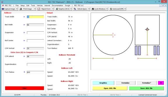
Figure 454

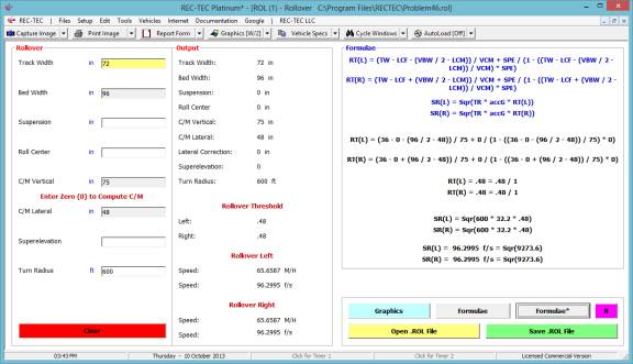
Example 2: A vehicle has a Track Width of 72 inches, a Bed Width of 96 inches, a Suspension of 4 inches, a Roll Center of 28 inches, a Vertical Center of Mass (C/M) of 75 inches, a Lateral C/M of 48 inches, and a Turn Radius of 600 feet.

What is the Rollover speed to the Right? What is the Rollover speed to the Left?

Figure 455

Figure 456

Example 3: A vehicle has a Track Width of 72 inches, a Bed Width of 96 inches, a Suspension of 4 inches, a Roll Center of 28 inches, a Vertical Center of Mass (C/M) of 75 inches, a Lateral C/M of 48 inches, a Superelevation of 0.06, and a Turn Radius of 600 feet.

What is the Rollover speed to the Right? What is the Rollover speed to the Left?

Figure 457

Figure 458

Example 4: Use the same data as Example 3 except - compute the trailer's center of mass using the following information:

 Unit Weight Vertical Lateral (Left to Right)

Trailer 12000 48 48

Load #1 9000 110 24

Load #2 22000 78 24

Load #3 18000 90 72

Figure 459

Figure 460 appears after accepting the Number of Loads in Figure 459.

Figure 460

Figure 461 appears after clicking on Execute after placing the data in Figure 460.

Figure 461

Figure 462 appears after clicking on Execute after placing the data in Figure 461.

Figure 462

Figure 463 appears after clicking on Execute after placing the data in Figure 462.

Figure 463

Figure 464 appears after clicking on Execute after placing the data in Figure 463.

Figure 464

Click on the Graphics button to bring up the display in 465.

Figure 465

Use the [Esc]ape key to bring up Figure 466.

Figure 466

Module 52: Heavy Truck – Weight & Balance

(Table of Contents)

Overview: This module computes axle weights and center of gravity for Articulated Vehicles based on information about Tractor, Trailer and Load.

At the REC-TEC pull down menu, select Heavy Truck > Weight & Balance and the Weight & Balance screen appears (Figure 467).

Figure 467

Required Input Data

Weight and Balance

· Tractor Weight – Weight of Tractor

· Steer Axle-CG – Distance: Steer Axle to CG of Tractor

· Steer Axle-5W – Distance: Steer Axle to Fifth Wheel

· Steer Axle-DA – Distance: Steer Axle to Drive Axle (Center of Duals)

· Kingpin-TA – Distance: Kingpin to Trailer Axle (Center of Duals)

Option 1

· Trailer Weight – Weight of Trailer Only

· Load Weight – Weight of Load

· Kingpin-CG(T) – Distance: Kingpin to CG of Trailer

· Kingpin-CG(L) – Distance: Kingpin to CG of Load

Option 2A & 2B

· Kingpin Weight (2A) – Weight on Kingpin

Or

· Kingpin - LG (2B) – Distance: Kingpin to Landing Gear

· LG Weight (2B) – Weight on Landing Gear

Required (2A & 2B)

· TL Axle Weight – Weight on Trailer Axle

All Examples: Tractor Weight = 16000#, Steer Axle to CG = 90 inches, Steer Axle to 5^th Wheel = 185 inches, Steer Axle to Drive Axle = 195 and Kingpin to Trailer Axle = 426 inches.

Example 1: Trailer Weight = 12000#, Load Weight = 40000#, Kingpin to CG(Trailer) = 375 inches, Kingpin to CG(Load) = 204 inches.

Figure 468

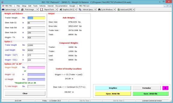
Figure 469

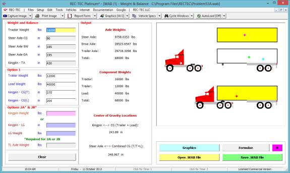
Example 2: Kingpin to Landing Gear (Trailer) = 50 inches, Landing Gear Weight = 25312#, Trailer Axle Weight = 26688#.

Figure 470

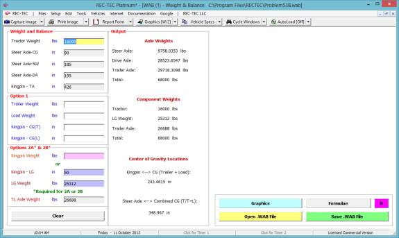
Figure 471

Example 3: Kingpin Weight = 22334#, Trailer Axle Weight = 29666#.

Figure 472

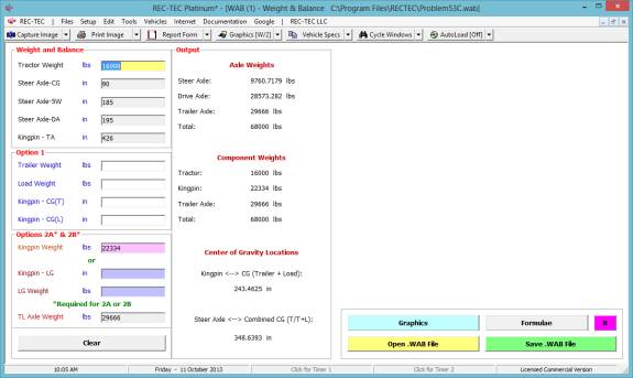
Figure 473

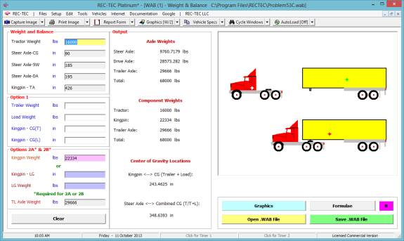
Module 53: Time - Distance – Time - Distance (EDM)

(Table of Contents) (Table of Contents)

Overview: This module computes basic Time and Distance information from data retrieved from Event Data Modules (cars and trucks) and formats it for enhanced examination by the Time - Distance Multiple Events module.

At the REC-TEC pull down menu, select Time - Distance – Time - Distance (EDM) and the Time - Distance – (EDM) screen appears (Figure 474).

Figure 474

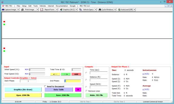
Required Input Data

· Speed (Initial) for Phase – from ECM, CDR or Railroad data recorders

· Speed (Final) for Phase – from ECM, CDR or Railroad data recorders

· Event End Time (for Phase) – from ECM, CDR or Railroad data recorders

· Start Phase (Controls Graphics and Data Table)

· End Phase (Controls Graphics and Data Table)

Example 1: Time starts at 0 seconds. Each Phase is 1 second.

1. Phase 1 - Initial Speed = 72 M/H Final Speed = 72 M/H

2. Phase 2 - Initial Speed = 72 M/H Final Speed = 68.5 M/H

3. Phase 3 - Initial Speed = 68.5 M/H Final Speed = 48 M/H

4. Phase 4 - Initial Speed = 48 M/H Final Speed = 31 M/H

5. Phase 5 - Initial Speed = 31 M/H Final Speed = 31 M/H

6. Phase 6 - Initial Speed = 31 M/H Final Speed = 14.5 M/H

7. Phase 7 - Initial Speed = 14.5 M/H Final Speed = 8 M/H

8. Phase 8 - Initial Speed = 8 M/H Final Speed = 2 M/H

9. Phase 9 - Initial Speed = 2 M/H Final Speed = 0 M/H

Figure 475

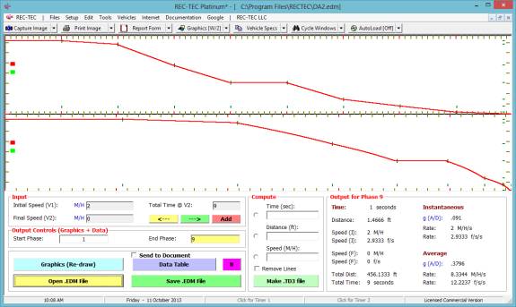
Figure 475 displays the screen when the last phase has been entered.

Figure 476

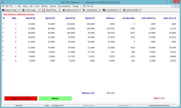
Figure 476 displays the module Data Table and with the data for each of the (9) phases. Placing a check in one of the boxes eliminates the entry from the computations. The program transitions from the last unchecked box to the next unchecked box. Figure 477 shows the Data Table with Phase 5 checked.

Figure 477

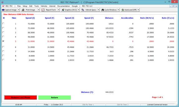
Figure 478 displays the Graphics on the EDM screen. Placing a check in one of the boxes on the Data Table eliminates the entry from the computations. The Graphics shows the transition from the last unchecked box to the next unchecked box. Figure 478 shows the transition from Phase 4 to Phase 6.

Figure 478

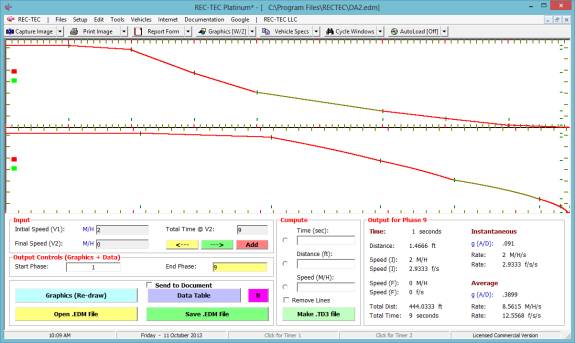
Place a time of 5-seconds in the Time box (Compute frame) and then click on the adjacent Radio button (Figure 478).

Figure 479

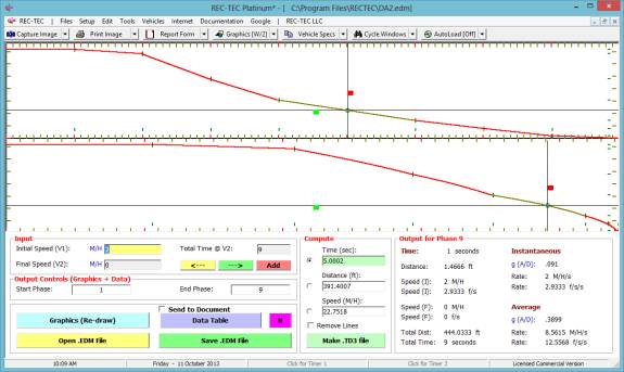
Figure 479 displays very thin crosshairs drawn on the screen along with a small circle on both curves. The data (Distance and Speed) are shown in the frame for the Time selected.

Figure 480

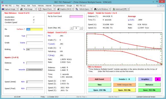
Pressing the Make .TD3 file creates a file named EDM.TD3 and starts the Time - Distance Multiple Events module. The file will automatically load as shown in Figure 480.

Figure 481

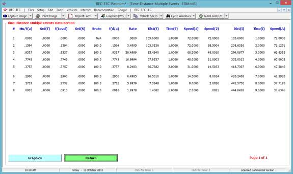
The data from the Time - Distance Multiple Events module as loaded from the EDM.TD3 file is shown in Figure 481.

Figure 482

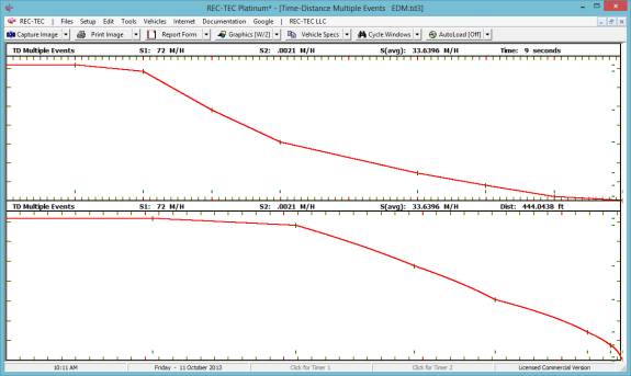
Figure 482 shows the Graphics curves drawn in Time - Distance Multiple Events (full screen).

Example 2: Using the intermediate computations from Time - Distance Multiple Events (Module 5, Example 1, Figures 62-69), the EDM module arrives at the same results allowing for the error involved in using four decimal places in the time and speed entries.

Figure 483

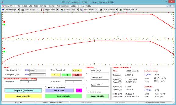
Figure 483 shows Example 2 run in the EDM module.

Figure 484

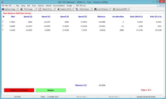
Figure 484 shows the Data Tables in the EDM module.

Figure 485

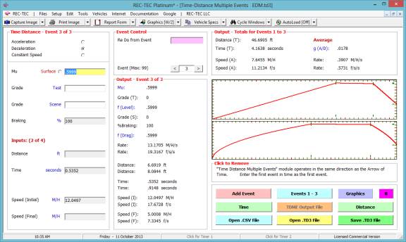
Figure 485 shows Example 2 run in the Time - Distance Multiple Events module.

Figure 486

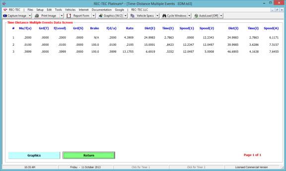
Figure 486 shows the Data Tables in the Time - Distance Multiple Events module.

Example 3: Using the intermediate computations from Time - Distance Acceleration-Transition-Deceleration (Module 7, Example 1, Figures 86-91), the EDM module arrives at the same results allowing for the error involved in using four decimal places in the time and speed entries.

Figure 487

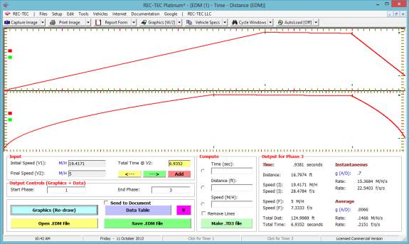
Figure 487 shows Example 3 run in the EDM module.

Figure 488

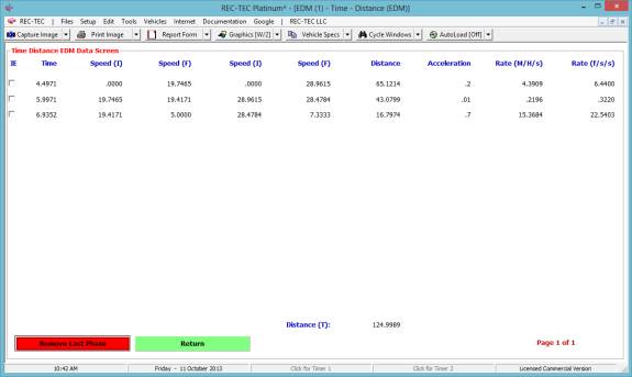
Figure 488 shows the Data Tables in the EDM module.

Figure 489

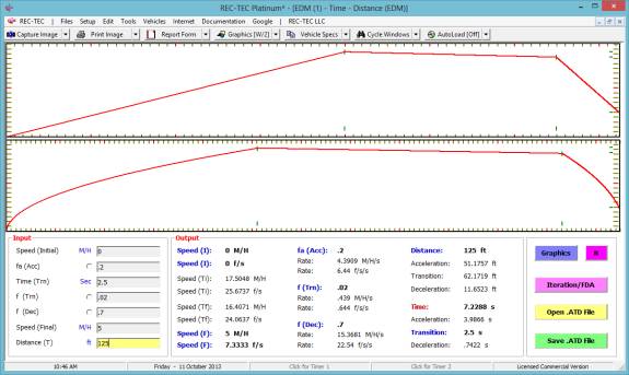
Figure 489 shows Example 3 run in the Time - Distance (Acc~Dec) module.

Example 4: The data for example 4 is shown in Figure 491.

Figure 490

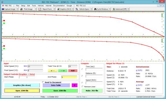
Figure 490 shows Example 4 run in the EDM module.

Figure 491

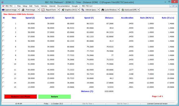
Figure 491 shows the Data Table for Example 4 in the EDM module.

Figure 492

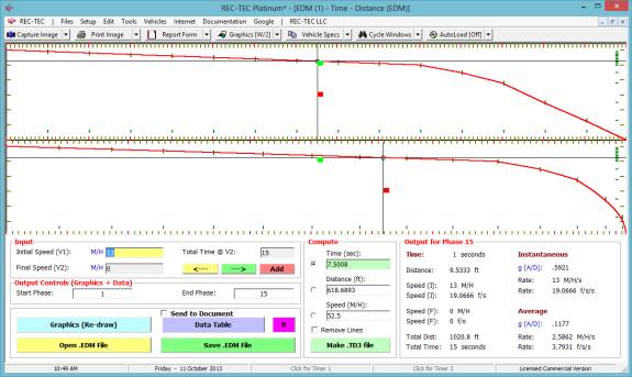
Figure 492 displays the crosshairs and small circles for 7.5 seconds in the EDM module.

Module 54: Time - Distance – V-TRAX

(Table of Contents) (Table of Contents)

Overview: This module animates up to four vehicles in various acceleration, deceleration or constant velocity scenarios while allowing two of the vehicles to execute turning maneuvers.

At the REC-TEC pull down menu, select Time - Distance – V-TRAX and the Time - Distance – V-TRAX screen appears (Figure 493).

Figure 493

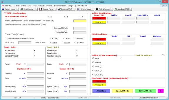
Required Input Data

This is the section of the program that is the most difficult to handle. Because each project is different, it is impossible to set up a neat “Problem” that can be illustrated here. Several different scenarios have been worked up as “sample” runs. There is a great amount of flexibility built into this section. It is suggested that you “create” a small problem with 2 vehicles, get them to do what you want them to do, and then start adding other vehicles to give the project more detail if necessary.

Please, do not start working with this section the night before. It takes a little practice to get good with this section and you will do much better if you are not working under the pressure of a deadline.

Project LTURN2:

This project has 2 vehicles. Vehicle 1 is in a complex swerve (turn) maneuver while accelerating from a stop. Vehicle 2 will decelerate to avoid collision with vehicle 1. This project will be described in detail on the next few pages.

Figure 494

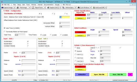
 The screen on the next page shows the animation run to completion.

Refer to the screen above for the following:

1. The total number of vehicles is 2.
2. Zoom and Offset distances are set and changed by zooming in or out and right, left, up and down positions while the animation is running.
3. Auto Time sets 1/10000 framing at ½ second before termination of animation based on time.
4. Terminating action at final speed would cause the vehicles to stop when they reach their respective final speeds.
5. Total Animation time has been set to 3.25 seconds.
6. Initial Time framing is 1/100^th of a second. The diagram is redrawn to show the movement of the vehicles for every 1/100^th of a second of (real) time.
7. Unit 1 will be accelerated using the data shown.
8. Unit 2 will be decelerated using the data shown.
9. Vehicles 1 & 2 are using Crush Files (imported) and drawn to scale (W + L are read from file).
10. The Lane widths are set at 12 and the offset on #2 is 0.
11. Vehicle 1 will initiate the acceleration immediately (0 PRT) and be 24 feet from the X (Center Reference Point of the animation.
12. Vehicle 2’ path is at 90 degrees to Vehicle 1’s initial path. It will start decelerating 2.3 seconds (real time) after the animation start. Vehicle 2 is 250 feet from CRP at the start of the animation.
13. Vehicle 1 will commence a .3g (perpendicular to initial path) accelerated turn to the top of the screen at 2.23 seconds after the animation starts and may continue for 100 feet lateral. The radius of the turn is maintained at the initial radius even though the vehicle is accelerating.

With this information in mind, view the animation, which is shown below run to completion at 3.25 seconds from start.

Figure 495

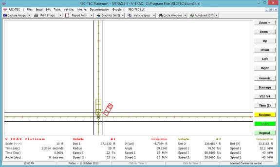
Project LTURN4:

This project has 4-vehicles. Vehicle 1 is in a complex swerve, return then swerve (turn) maneuver.

Figure 496

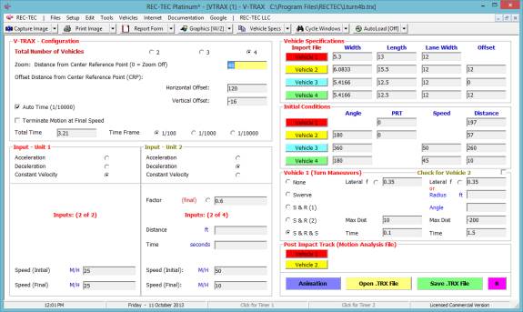
Figure 496 displays a 4-vehicle configuration with two of the vehicles in acceleration.

Figure 497

Figure 497 displays Vehicle 1 turning north behind Vehicle 3 blind to Vehicle 2.

Figure 498

Figure 498 displays Vehicle 1 at maximum engagement with Vehicle 2.

Figure 499 

Figure 499 displays Vehicle 1 engaging Vehicle 2 in collision.

Figure 500

Figure 500 displays Vehicle 1 at maximum engagement with Vehicle 2. Display is zoomed in on area of impact (AOI).

Figure 501 

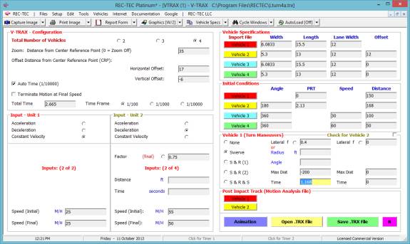
Figure 501 displays a 4-vehicle configuration with two of the vehicles in acceleration. Vehicle 1 is in a turn and Vehicle 2 decelerating.

Figure 502

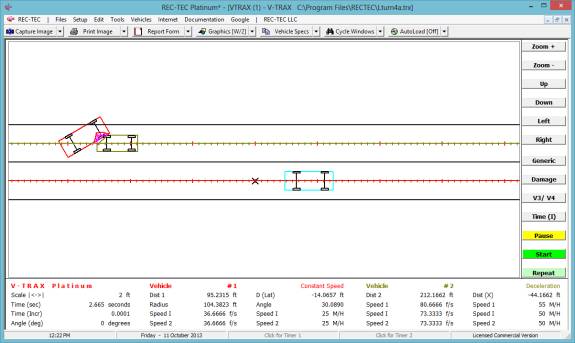
Figure 502 displays Vehicle 1 at maximum engagement with Vehicle 2.

Figure 503 

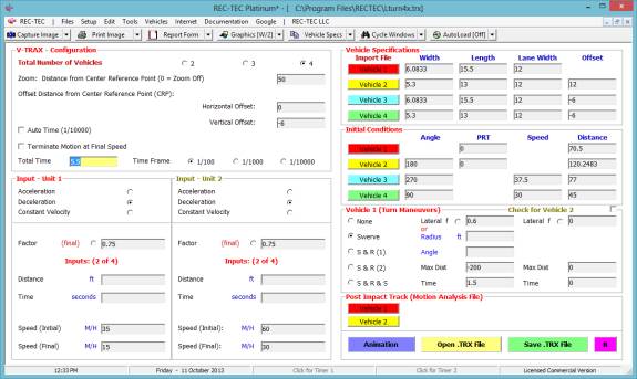
Figure 503 displays a 4-vehicle configuration with all four vehicles going through an intersection together with Vehicle 1 is in a turn.

Figure 504

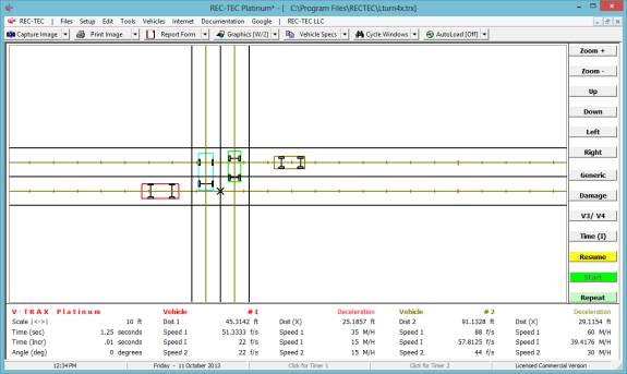
Figure 504 shows Vehicle 3 and Vehicle 4 in the intersection. Vehicle 1 and Vehicle 2 are approaching the intersection.

Figure 504B

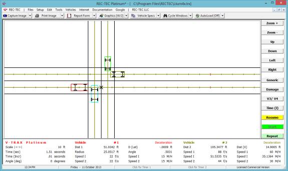
Figure 504B shows all four vehicles in the intersection at the same time. Vehicle 1 is about to execute a turn.

Figure 505

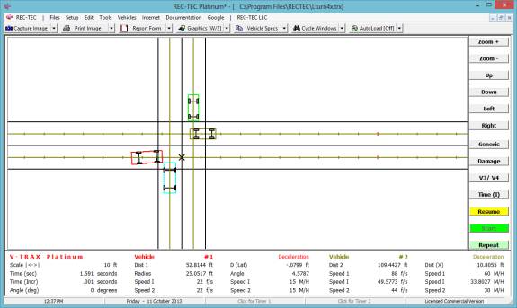
Figure 505 shows three of the four vehicles still in the intersection. Vehicle 1 is starting to execute a turn.

Figure 506

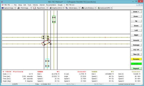
Figure 506 shows two of the four vehicles still in the intersection. Vehicle 1 is executing a turn.

Figure 507

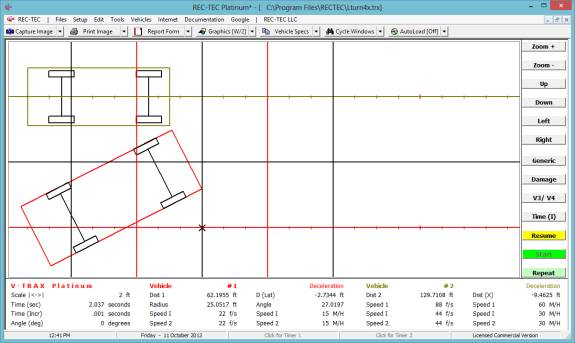
Figure 507 shows two of the four vehicles still in the intersection. Vehicle 1 missed Vehicle 2.

SMAC Primer

(Table of Contents)

By George M. Bonnett JD

Welcome to SMAC-RT and this Primer on SMAC in general. This new version focuses on SMAC-RT and uses screen captures from SMAC-RT.

SMAC-RT is the property of REC-TEC LLC and is free to all REC-TEC users with a current Platinum option. We will continue to upgrade this basic version of SMAC. The SMAC engine we are using is a modification of the 1997 version that Calspan obtained from UMTRI. In its original form as downloaded from Calspan, it was unusable. It has been modified slightly to make it functional and to produce the required/desired output files.

There are some idiosyncrasies associated with this particular version:

1. Print Output timing is not totally controlled by the Print output time entered in Card 1. The timing sequence shifts during the collision phase, and returning after collision.

2. Rear wheel steering is not controlled by Cards 4 and 5, but by Cards 10 and 11. The forces in Cards 10 and 11 can be toggled On/Off using the green/gray Vertical bars (even in the Evaluation copy) creating an entirely different scenario.

3. Wheel (Torque) Forces may be entered by the traditional method of using a percentage of the weight on each wheel multiplied by the friction factor. Alternatively, the program interface will compute the information if a number between –1 and + 1 is used for braking/acceleration.

4. Wheel Forces and Steer Angles can be entered by either a fixed time interval, or by using a variable time interval (number of entries). With the Variable Time Interval a Checkbox is Enabled permitting the use of the Collision Detect feature for that wheel. Collision Detect holds a change spanning the time before and after collision from ramping up from Collision to the time frame immediately after Collision detection.

5. Files are “Saved” and “Opened” using the .Si5 format. The file created by the interface to run SMAC-RT is “Input.DAT.” This file is formatted to work in the SMACRT.EXE engine doing the majority of the number crunching necessary for the Graphics and Animation output.

Please remember that SMAC could be a very dangerous tool in the hands of the un-educated or un-scrupulous reconstructionist. It is NEVER the first tool used in a reconstruction. It is the last. It helps refine computations and calculations based on physical evidence.

Hopefully by making the program free, it will encourage more facilities to provide instruction on SMAC and therefore encourage users to purchase SMAC programs that go far beyond the basic features offered by this variant.

Here are some tips to help get you started (you may want to print this page so you can follow the steps):

1. When selected, the SMAC-RT module should automatically load the file Sample3.Si5. The inputs in the left most column, should be headed by a block that is labeled “Default.” In the lower right screen quadrant, you should see a block labeled “SMAC-RT.”

2. You might want to go “Full Screen” with the program in order to see all of the features. Now look on the Right side of the screen and find the Wheel Forces section. Click on the two vertical Green bars, disabling the braking on the vehicles (letting them reach their target blocks). You may want to play with the Braking and Steering later on, turning them on/off for the different vehicles. This, and the instructions following, are applicable to both the licensed and Evaluation copies of the program.

3. Click on the red “Run” button. A message will appear allowing several options for the LAMBDA value (Card 13-3). For this run, select “No.” This will run the SMACRT.exe engine and then bring up a panel showing the output file that may be used for data or high-resolution animations, or by REC-TEC to display both Graphics and Animations.

4. Click on the Animation button at the bottom of this panel. This will start an animation that should show a 4-second animation. The program automatically goes to Zoom Extents for the problem.

5. In the bottom-center of the screen, there are eight buttons and a checkbox (toggles rest positions on/off). The fourth button will be selected. Place you cursor on the different buttons and you will see that they describe different modifications to the animation. Select the seventh button. You should see two vehicles on the screen. They are not moving. Click again on Zoom Extents. The two vehicles now fill the screen. Press the “+” key (Shift + if you don’t have a number pad) and you will see the vehicles advance towards each other in the selected print output interval.

6. On both the right and left upper corners of the screen, you will see four blocks labeled “aV” (acceleration vector), “vV” (velocity vector), “CG” (center of gravity trace), and “TT” (Tire Trace) for Vehicles 1 (Left) and 2 (Right). Try turning on all of the Vectors.

7. Use the Plus key to advance the vehicles into the collision. You may also use the minus (-) key to back up the vehicle to the pre-collision positions. If you have repeat turned on for your keyboard, you may simply hold the key down to step the animation.

8. Right clicking on the mouse will start the animation. Let it run until it stops (off of the screen). Click on Zoom Extents again and then right click the mouse. The animation will start again. It may be paused (and re-started) by using the right mouse key or the spacebar.

9. The blocks at the top of the screen will let you move the display right, left, up, and down. It will also let you zoom in or out on the display. One button will reset the animation parameters, and others will let you alter the speed of the animation. There are buttons to shift the orientation clockwise and counter-clockwise and even a button allowing the animation to repeat. Clicking “R” (Repeat) or “Dsp” (Display All modes) to see various options randomly selected.

10. If you select the 8^th Animation button (bottom center) and then select either the 6^th or 7^th button, the program will not clear the screen between runs UNLESS you use the Plus or Minus keys to Step the animation for one time increment or more.

11. When you have finished exploring the animation variants, press Escape on your keyboard. Now Click on Graphics. There are all sorts of displays and curves for acceleration to velocities. Check them out on your own, noticing that you can select either vehicle for the displays and that the curves can be “timed” − Enjoy!

Congratulations! You finally made the big move to a SMAC program. Now the fun (and the learning) begins. Just make sure that your computer meets the specifications required by the program and that you have enough room on your hard drive to install all of the features you require.

The REC-TEC program contains a SMAC program called SMAC-RT. The SMAC-RT program works as an evaluation program unless your license permits you to use the full program. The Sentinel.exe file is the licensing file for both the REC-TEC Program and the SMAC-RT program. In order to use the SMAC-RT program your Sentinel file must include a current Platinum Option. SMAC-RT requires the Platinum option. This will allow all of the installations permitted under your license to run the licensed SMAC-RT software.

The SMAC-RT program in REC-TEC is our model. Clicking on REC-TEC on the upper navigation bar on the main screen causes the dropdown menu to appear. At the bottom, we see the SMAC selection.

Figure 508

Clicking on SMAC brings up the SMAC-RT screen (Figure 509).

Figure 509

This may seem confusing, even mind-boggling! Be patient, the program is actually rather simple. It is setting up two cars to crash into each other. We all know cars, right? You just have to learn the way the inputs for each car are arranged and a little about the inputs.

Several steps are key to understanding how to setup and run this program. With any new toy, or tool the first steps always seem the hardest. The program has sample case studies that can be loaded and run showing the data and graphics produced by SMAC. Click on the Open .Si5 File button.

A dialog box (Figure 510) appears showing the standard windows file selection dialog box. Each of these files is a sample smac input file. As you new files are created, this dialog will display filenames. Select the filename Sample3.Si5.

Figure 510

Opening the Sample3.si5 file in SMAC-RT (Figure 511) replaces all of the numbers in the opening data screen. There are quite a few zeros on the screen, and it has at least one blank box. For those users new to SMAC, it can be a confusing bunch of numbers and blocks. That is OK. Soon it will all make sense!

Figure 511

This is the basic control point for setting the parameters for running a SMAC problem. Instead of explaining all of the blocks at this point, see what it can do. In the lower right section of the screen are the main control buttons for the program. The Open.Si5 File button got us to this point. Press the red Run button and jump right into the thick of things. After a slight pause a new screen will appear (Figure 512).

Figure 512

As reported in Figure 512, the suggested maximum value for Lambda is 8.5 and the suggested minimum value is 4.4. The value entered is 12 as shown in the (dark red) input textbox, and triggering this message.

The McHenry (m)SMAC programs automatically lower a value over the Maximum (8.4 for this problem) to the Minimum (4.4 for this problem) for the computations, placing a note in the output files stating the value has been lowered. REC-TEC (SMAC-RT) displays the above message, giving the user control (and knowledge) of the input used in the computation. This value can have a dramatic effect on the outcome.

For the purpose of this exercise, select the “No” response. This block (Figure 512) will not appear if the values are between the minimum and maximum.

Figure 513 (Datasets Selection is displayed)

Figure 513 is not exactly the rush that was anticipated.

Just as we are taking baby steps right now, so is the program. Only the program did more than you realize. It was also generating pages and pages of data and over a dozen files that it placed in the directory. These files are the result of running the Simulation (number crunching) side of the program and are the documentation that you will need to effectively use the program in any litigation – civil or criminal.

The Datasets are now shown on the screen (Figure 513). This will let us view what the program was doing when we pressed the Run button. Several different files were created during the “Run” phase that may now be reviewed. In addition to echoing the input data, these files will show all of the computations that the program has made showing the instantaneous speeds, distances, forces, accelerations (linear and angular), changes in velocity (delta V), damage, steer and tractive forces for the vehicles as well as other data that may be useful in your case. All of these files are available and may be added to the report.

A note of Caution: The files produced are for the particular problem being run. The program writes over these files as new problems are run. If you need to go back and retrieve a file that has been overwritten and not saved in a report, it will be necessary to re-run the original problem. The main .Si5 file is not overwritten unless you purposefully overwrite it using the Save button.

The Graphics button will bring up Figures 514 (without Card 80 Damage shown) and 515 (with Card 85 Damage shown). These figures show the predicted SMAC damage when the SMAC radio button is selected.

Figure 514

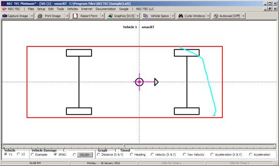
Figure 515

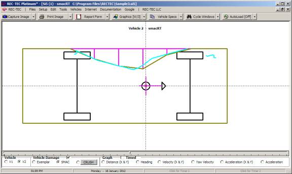
These screens show both vehicles, including the damage pattern predicted by the program. This is not the damage pattern input into the program using the Options button. In fact, this has nothing to do with the damage pattern input into the program as “target damage.” This is program predicted damage. (The Options button and the “target damage” will be discussed later.)

In addition to the vehicles there are Graphics screens showing various information about this particular simulation. There is a wealth of information available using this section. It is a distillation of what occurred during the simulation.

Figure 516

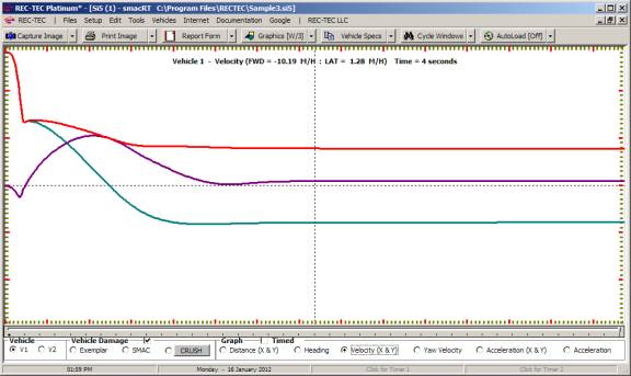
Figure 517

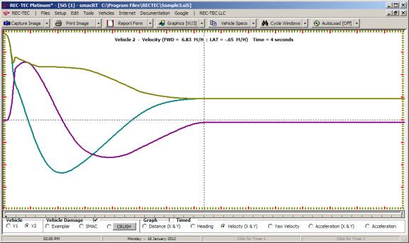
Pressing the Escape key (or the center wheel on the mouse depending upon the mouse setup the user is returned to the screen shown in Figure 518.

Figure 518

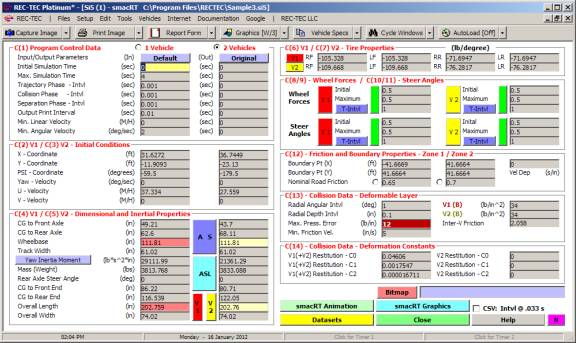
This is still not the kind of thing that will get the average cynic to hyper-ventilate, but there is still one more button to go – Animation (Figures 519, 520, and 521).

Figure 519

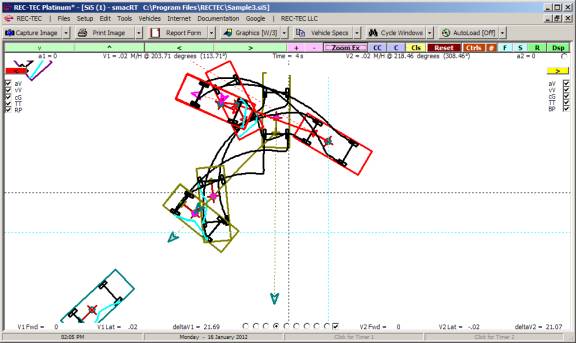
Figures 520 and 521 display the modified run produced by changing the Output Print Interval C1) and the clicking on the green Wheel Forces buttons C(8/9) in Figure 518. This effectively slows the animation and disables the input Wheel Forces.

Figure 520

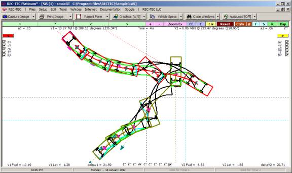
Figure 521

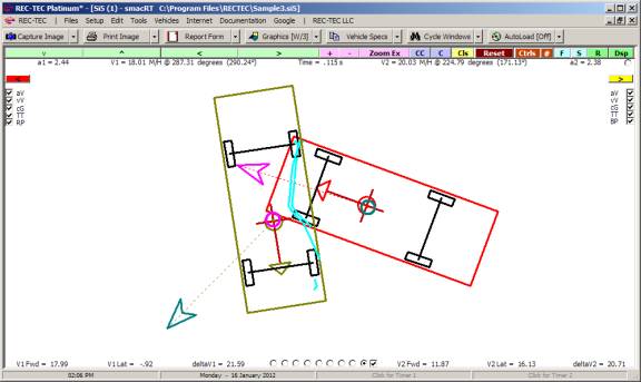
I can hear the purists screaming from here. Animation? SMAC is a simulation program. How can you talk animation when we are dealing with a simulation program? The truth of the matter is that both terms are correct. SMAC as a totality is a simulation program. In fact, the term “SMAC” refers to Simulation Model of Automobile Collisions, and was created by Raymond McHenry and his crew of merry men in response to a 1970 National Highway Traffic Safety Administration (NHTSA) sponsored research project.

The Run Button initiates the simulation. The actual program run at that time is SMACRT.exe and it does the simulation, which produces the data files that have been previously discussed. The Graphics Button reads some of these files to produce the graphics. The Animation Button reads the files and produces the animation from the points specified in the files. So, while SMAC is a simulation, clicking on the Animation button produces an animation, not a simulation. Press Animation and…(Figure 522)

This is only the beginning.

Figure 522

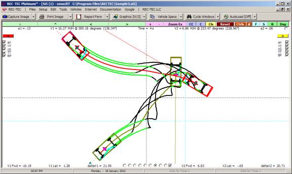
The next few pages show screen captures all using the same basic setup in Sample3.Si5. The difference between Figure 522 and Figure 520 is that the Steer angles for the right and left front wheels in Figure 518 C(10/11) were changed to 0 degrees in the animation for Figure 524 by clicking on the Green bars.

Notice that this minor change resulted in an entirely different post impact run out of the vehicles. The secondary slap during the collision (Figure 523) does not occur in Figure 524. The Target blocks are clearly visible in Figure 524 even though the final position for the four (4) second run in Figure 524 has the vehicles miss their mark with the steer angles disabled. Figures 525 and 526 show close-ups of the secondary slap with the Vector option turned on.

Figure 523

Figure 524

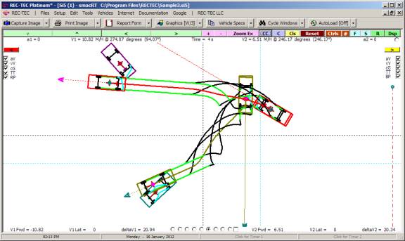
Figure 525

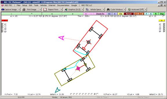
Figure 526

This is what SMAC does. It takes the inputs entered and models the actions and reactions of the vehicles using the laws of physics. By changing the inputs, the accident changes because the vehicles react differently to the forces acting upon them before, during and after the engagement phase of the incident being modeled.

Now that we have a basic feel for what SMAC is, and to some extent how it operates, we need to go back to the beginning and see what makes up the individual sections (cards) that make up the inputs screens and discuss how these inputs influence the final product. Once the inputs are understood working different types of problems will be much easier.

In the final section, different types of problems will be presented and using a step-by-step approach the information will be entered into the input screens and tested. The inputs will then be modified until the results displayed match the results of the incident we are trying to model as closely as possible.

With a thorough understanding of how the program works and the inputs that go into modeling the pre-collision, collision and post collision phases of the accident, SMAC will become a valuable tool in understand collisions. SMAC cannot replace the meticulous investigation and evidence gathering at the scene of an accident. It will not solve the accident for us by simply plugging in a few pieces of information gathered at the scene.

What SMAC will do is test our theories of how a particular accident happened. It will test and help us check and refine some of the data and preliminary conclusions arrived at using that data.

Now that we have seen what SMAC does, let us look at what goes into making it do it. Figure 19 is the primary input screen with the Sample3.Si5 file loaded. The frame at the upper left of the screen, labeled C(1) - Program Control Data allows setting up for one or two vehicles. The C(1) refers to Card 1 of the cardset that makes up the input file.

Figure 527

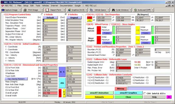
Figure 528 is a printout of the Sample3.Si5 file. A close inspection of Figures 531 and 532 will show the relationship between the cardset (Figure 528) and the data in the individual card frames in Figure 527.

In the early days when SMAC ran only on mainframes, punch cards were used to feed the data into the computers. Using the card format not only simplifies the inputs for the program, it makes for compatibility among the various versions of SMAC.

Card 1 or C(1) sets the timing for the program and the parameters under which the program will end. The data names for the individual inputs are displayed by placing the cursor on the entry block for the information.

Figure 528

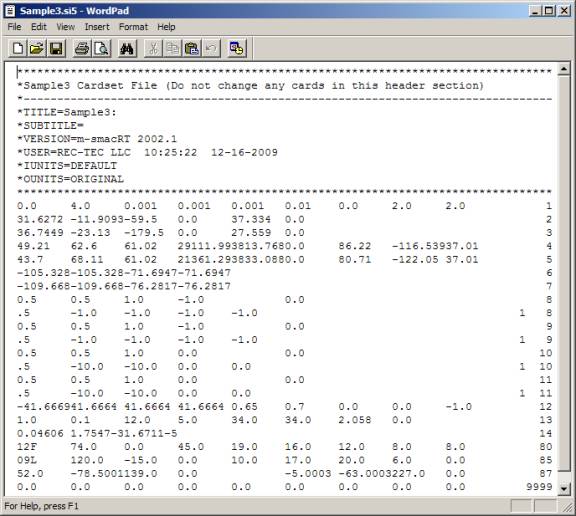
The above input file is the cardset that comprises data making up the Sample3.Si5 scenario.

Before moving on to setting up different scenarios, let’s take a look at some of the other features and widgets offered on the main SMAC-RT screen (Figure 527) that will play a part in producing the final output.

More Buttons and gadgets

The only button not discussed is the Options button. Clicking on the Options button modifies the screen to that seen in Figure 529.

Figure 529

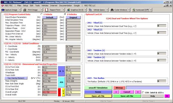
Figure 530

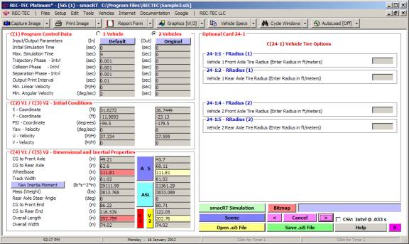
Figure 531

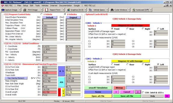
Figure 532

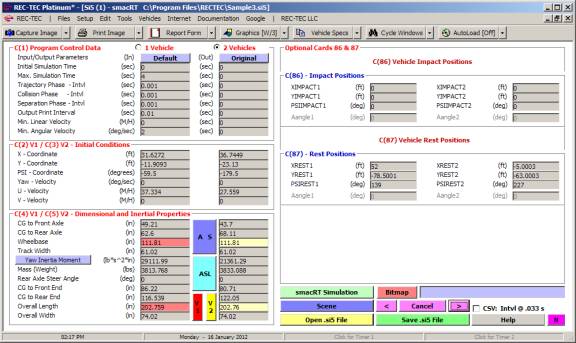
Cards 80, 85 and 87 on this screen deal with targets. They have nothing to do with the actual simulation or animation of the data within the datasets other than to act as targets.

Cards 80 and 85 are the targets for the damage to the respective vehicles. Cards 86 and 87 are the targets for the Impact and Final position for the vehicles.

What do we mean by targets? A target is something we aim at in various sports. In SMAC it is the result we are aiming for at the end of the run. In the case of the damage, this is the location and extent of damage that we are trying to have the program produce. In the case of the final rest positions, this is where the vehicles actually came to rest in the accident. We are trying to see how close our SMAC model comes to the target damage and rest positions.

Notice that there are Vehicle Damage Classification codes. These are the codes produced by the program following the laws of physics for the information supplied. They may or may not be the same as the user entered codes in Cards 80 and 85. Likewise, we cannot specify where (position-wise) either of the vehicles is to finally come to a stop. The user enters certain parameters in time, speed and rotation that will terminate the computations and animation, but not the actual positions. The target positions are the positions where the vehicles in the incident came to rest.

In the upper right of the screen, (Figure 527 – Card 1) two blocks control the Input and Output settings for the program. The settings are Original, Default, and Metric. The leftmost button controls the Input settings for the program. Changing this setting will change how the data is shown on the screen.

Caution should be used when changing to Metric as the inputs are truncated to the decimal setting selected for the program. This change can have a small change in the files (Cards) that are used to create the Graphics and Animation for the program.

Above these two blocks are also two radio buttons that will configure the program for either one or two vehicles. When the radio button is selected showing only one vehicle the second vehicle information is not only removed from view but is not sent to the datasets and therefore not be sent to the Graphics and Animation programs.

Figure 533 shows the Single Vehicle Interface.

Figure 533

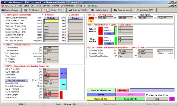
Selecting the 2 Vehicles radio button will restore the screen to the configuration in Figure 527.

In the frame for Cards 4 and 5, the block labeled Inertia Moment (Yaw) is actually a button. By clicking on this button a frame appears (Figure 534) that calculates the Yaw Moment of Inertia for the dimensions in the inputs for both vehicles. These values can be transferred to the respective input blocks for the vehicles.

Figure 534

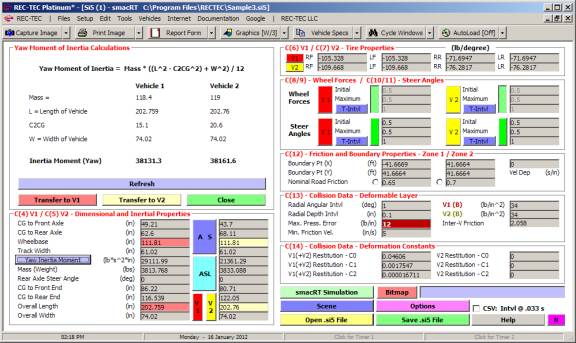
Down the center of the input blocks for Cards 4 and 5, two large buttons will allow the user to import the dimensions for different vehicles. The buttons are labeled AS (AutoStats) and ASL (AutoStats Lite) Clicking on AS will bring up the frame shown in Figure 535.

Figure 535

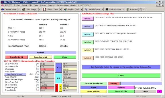
The new frame shows the Vehicle Exchange Files that can be set up in AutoStats. Once a Vehicle’s data has been pulled up in the AutoStats program, it can be transferred to the Vehicle Exchange file by going to the last page of the data and pressing on selecting E for Exchange file (Figure 536).

Figure 536

Figure 537

Once the vehicle is placed in the Vehicle Exchange Files, the REC-TEC program can call them up and then automatically transfer the data into the SMAC-RT section (or the Crush section).

Clicking on one of the vehicles displayed will transfer the data to REC-TEC and set up the frame for Cards 4 and 5 as shown in Figure 28. Selecting V1 will then transfer the information to the input blocks for that vehicle as shown in Figure 35. If the CNX button is selected, the data will not be transferred and the frame will return to its normal configuration (Figure 527).

Figure 538

Figure 539

Below the AS and ASL buttons are 2 buttons labeled V1 and V2 with a slider bar directly below them. Clicking on these buttons will bring up a scale diagram of the vehicle based on the dimensions displayed in the input blocks.

Before displaying the Graphics for Vehicle 1, the setting for REC-TEC Graphics will be changed to a background color of Windows Default and for Wide Lines using the Graphics Icon directly below the main menu resulting in the display shown in Figure 540.

Figure 540

Selecting the ASL button brings up the AutoStats Lite page (Figure 541). This selection does not require the user to own AutoStats as the Vehicle Exchange Option does. If AutoStats is not installed on the computer then this is the only option for vehicle dimensions that will appear. AutoStats Lite is built into the REC-TEC program and is available to all users.

Once the Make, Year and Model have been selected, the data for that vehicle will be displayed on the form. In addition to the data, a block will appear that will return to SMAC-RT with the data (Figure 542). Clicking on this block will cause the AutoStats Lite Page to disappear and bring up the SMAC-RT screen as displayed in Figure 543.

Figure 541

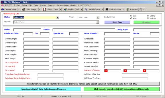
Figure 542

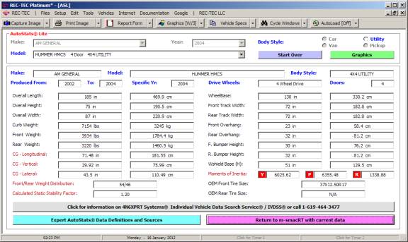
Figure 543

Figure 544

Clicking on the V2 Button will transfer the data to the input blocks on the SMAC-RT screen as shown in Figure 544.

Clicking on the 2 Button will bring up the REC-TEC graphics screen showing Vehicle 2 scaled to the dimensions shown in the input blocks (Figure 545).

Figure 545

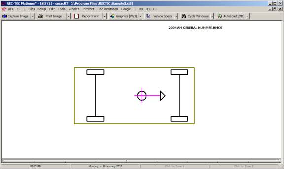
Using the data transferred to the SMAC-RT screen using the AutoStats/AutoStats Lite files as the Run button is selected will change the outcome of the simulation as reflected in the Run animation and the Graphics and Animation as displayed in Figures 546 through 548. Changing the dimensions of the vehicles, especially the masses of the vehicles even though the rest of the data remains the same has a dramatic effect on the simulation. Change Radial Angular Interval to 2.

Figure 546

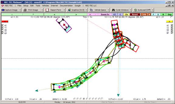
Figure 547

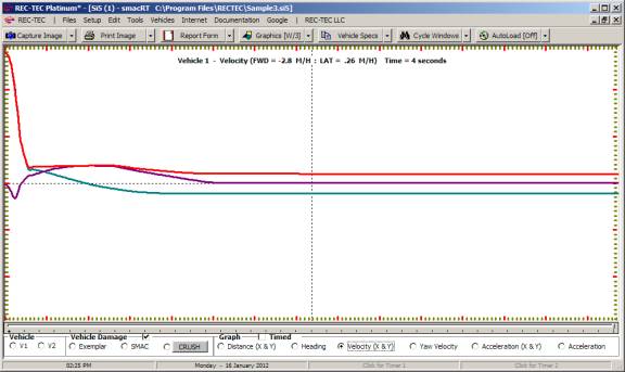
Figure 548

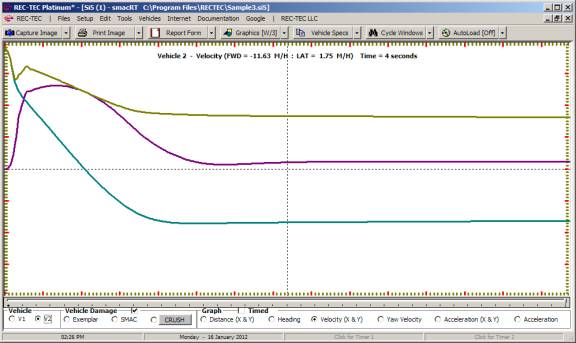
REC-TEC LLC has made a commitment to continually improve and upgrade their products keeping their users supplied with the very finest accident reconstruction tools available. Upgrades will refine and enhance the already extensive capabilities of the SMAC-RT program.

Wheel Forces and Steer Angles - Cards 8, 9, 10 & 11

Figure 549

Cards 8, 9, 10, and 11, as seen on Figure 549, need a bit of explaining beyond the scope of the Help files. Some of the boxes and associated features may be confusing at first.

Cards 8 and 9 deal with the Wheel Forces for vehicles 1 and 2 respectively. They are the tractive forces that control acceleration (positive values) or deceleration (negative values) acting on the vehicles. Manipulating these values for specific periods controls the acceleration or deceleration of the vehicle.

Wheel (Torque) Forces may be entered by the traditional method of using a percentage of the weight on each wheel multiplied by the friction factor. Alternatively, the program interface will compute the information if a number between –1 and + 1 is used for braking/acceleration.

Wheel Forces and Steer Angles can only be entered by time interval, not by using number of entries. Older .Si5 files if not in the time interval format must be converted.

Associated with the individual sections for both Wheel Forces and Steer Angles on each vehicle there are rectangular green bars. These green bars indicate that the program is setup to utilize the values for these entries. Clicking on these bars will change the color and detail of the bar to indicate that the values for the chosen vehicle will be disregarded when the program is run. Figure 39 shows the Wheel Forces as disabled. This allows the user the flexibility of turning off these values and comparing the runs with and without the features engaged.

Now that we have a better understanding of the gadgets in the blocks controlling the Wheel Forces and Steer Angles, look at the actual numbers that are placed in the cards for the individual vehicles. Figure 40 shows the single entry for Wheel Forces for Vehicle 1 and Figure 41 shows the Steer Angles over the time at the prescribed interval for Vehicle number 2. This is where we insert or modify the actual values that go into the computations and animation/simulation.

If the user enters values from –1 to +1, the interface will automatically compute the appropriate values to enter into” INPUT.DAT” for Maximum Braking or Maximum Acceleration for the entered surface friction. It is up to the user to determine the correct values to enter depending on the situation being modeled.

Figure 550

Figure 551

The Fun Begins – Setting up out first problem.

So how do we start to set up a problem?

Once the SMAC section is opened, loading a recently included file named Default.Si5 will give us a jump-start in setting up a problem. If Default.Si5 does not appear on the file list, simply create one using the values shown in Figure 552 and save it to the folder. This file will set up some common values that can always be modified as your particular problem dictates.

Figure 552

As can be seen some common values have now been set (or partially set) for Cards 1, 6, 7, 12, 13 and 14. This will speed up the process for creating out first problem. Notice that the screen is set to use Default as the Input and Output units involved in this problem.

With Card 1 preset, Cards 2 and 3 can now be used to set up the problem. Setting up the Initial conditions for the vehicles can be the most difficult part of the process. While the desire is to show as much as possible dealing with the pre-impact phase of the collision, if we start the vehicles too far from each other initially, they may not even collide. One of the biggest tricks in setting up a SMAC run is to set up the vehicles so that they are fairly close to impact and do the post-impact phase first so that it closely resembles the data we have. Once that is set, work on the pre-impact phase of the collision becomes less of a nightmare and the vehicles can be backed away from impact.

Our problem will have a 2003 Ford police unit traveling at 35 m/h from west to east (90 degrees) when it is struck by a 2002 Chevrolet Z06 Corvette traveling at 30 m/h from south to north (0 degrees). Both vehicles will be positioned 50 feet from impact Autostats was used to get the data for the vehicles. The resulting configuration is shown in Figure 553. The SMAC Animation is shown in Figure 554.

Figure 553

Figure 554

Wow, with just those few entries we staged a collision in a successful SMAC run.

Notice that while the X and Y values for the position of the cars is measured “globally” using the X and Y for the scene (world) that the U and V velocity components are local to the vehicle. Understand this and half of the battle has been won in working up SMAC runs.

For our problem, the police unit (#1) is struck in the right front wheel with the damage centered on the wheel. Since we are sure of our impact speeds from our calculations, how do we get the vehicles to hit so that the position of the collision damage in SMAC matches the damage resulting from the real world collision.

With the speed set, the only way is to change the distance from impact of the vehicles. If the Vehicle 2 X-coordinate is changed to –10 and the Y-coordinate is changed to 17 feet the vehicles strike each other in the correct location as can be seen in Figures 555 and 556.

Figure 555

As will be seen in Figure 556 and 558 (Enlarged) something very interesting happens. The vehicles now have a secondary slap involved in the collision. The only thing changed was the distance from impact and as can be seen, the post-collision actions of both of the vehicles are drastically changed. This is the power of SMAC. It uses the laws of physics to compute the motion of the vehicles.

Please take note that by stepping through the Animation we discover that impact for this collision occurs at 0.213 seconds into the animation. This time will become important when we start repositioning the vehicles before impact.

Figure 556

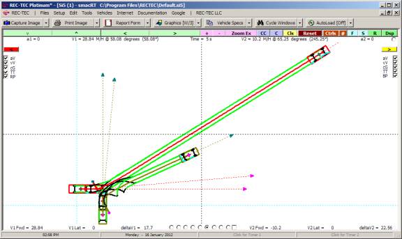
Figure 557

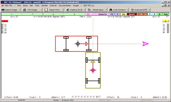
In order to be able to work on this particular scenario in the future, go back to the main SMAC screen and save the file. Name the file Problem45.Si5 so that it can be called up later without having to type the information in all over again.

Figure 558

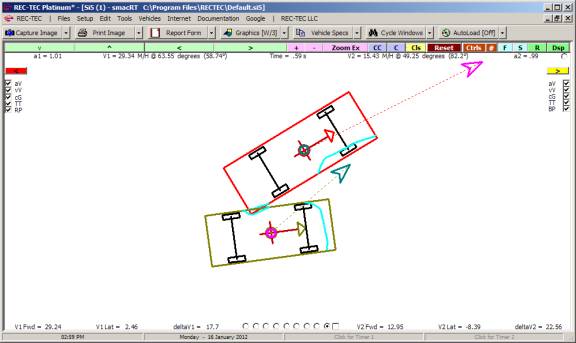
Set the braking due to damage on Vehicle 1 to reflect the locked brake on the front right wheel. Impact starts at .213 seconds. Getting the drag to come on between 0.213 and 0.215 seconds requires two entries for the braking. The entries are at 0.213 seconds and 0.215 seconds. This has the effect of ramping up the braking from zero to full braking in the 0.002-second period between 0.213 and 0.215 seconds.

Figure 559

With these changes in place, (see Figure 559 – Vehicle 1 entries) the effects can be seen in Figure 560. Because we are dealing with braking or deceleration, the value has a negative sign. Note that with the SMAC-RT, we can enter the torque value or the braking based on -1 being full lockup.

Figure 560

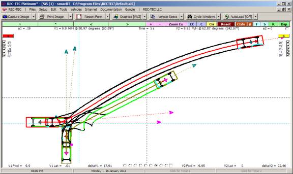
Assume that the steering of vehicle was also changed to positive 10 degrees during the impact. This change is shown in the graphics displayed in Figure 561 A, B & C. It also shows very dramatically, why linear momentum angles are not measured to point of rest.

Figure 561 A

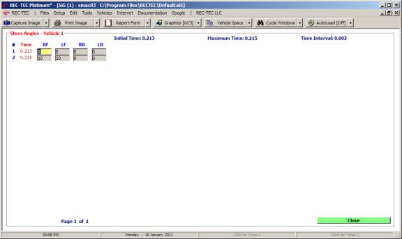
Figure 561 B

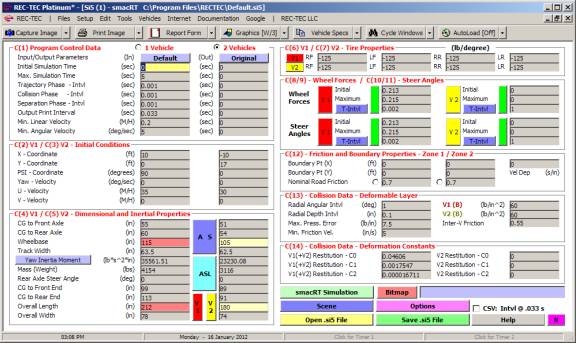
Figure 561 C

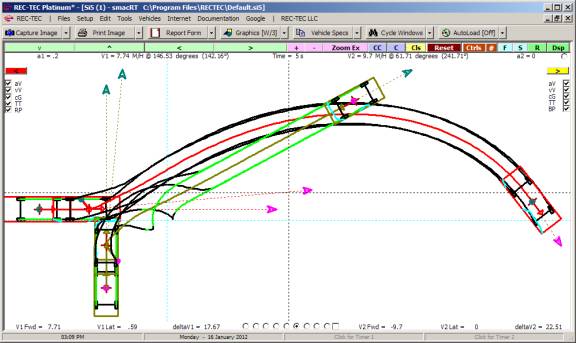
If we need to show more pre-impact tracking of the vehicles some adjustments are needed. Using a minimum distance before impact of 50 feet for (CG) Vehicle 1, what must be changed in the problem?

If Vehicle 1 is traveling at 35 miles per hour or 51.3333 f/s, what needs to be changed to have Vehicle 1 start at 50 ft before impact?

In order to visualize the linear relationships a little easier, it may help to have the collision occur at the intersection of the X and Y-axes. Changing the Vehicle 1 X-coordinate to zero and the Y-coordinate to –17 and the Vehicle 2 X and Y-coordinates to –20 and 0 respectively accomplish this in our problem. These changes are reflected in Figure 562.

Figure 562

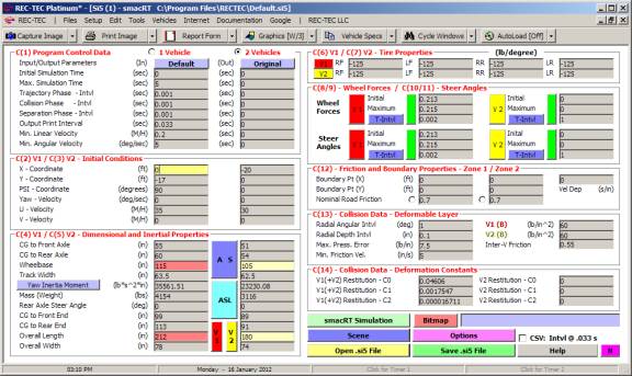
With these changes in place, the graphics diagram now has the X and Y-axes (Light Blue) as shown in Figure 563.

Figure 563

With these changes in place, the position of Vehicle 1 at impact is –6.07 feet. This can be read from the V1PVA.DAT file using 0.213 seconds as the time of Impact. In order to increase this to 50 ft from impact requires a change of 50 feet to a position of –56.07 feet on the Y axis.

It takes 0.974 seconds for Vehicle 1 to cover 50 ft. Vehicle 2 covers 42.857 ft. in 0.974 seconds. Vehicle 2 at impact is at –10.63 feet from the Y-axis. We must move Vehicle 2 to a position –53.487 feet from the Y-axis. These are the figures needed to alter the program to reflect the changes necessary. Vehicle 1 is now 50 feet from impact and Vehicle 2 is 42.857 ft from impact. These changes are shown in Figures 564 and 565.

It is imperative that the times for Card 8 and Card 10 be changed as seen in Figure 564.

Figure 564

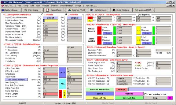
Figure 565

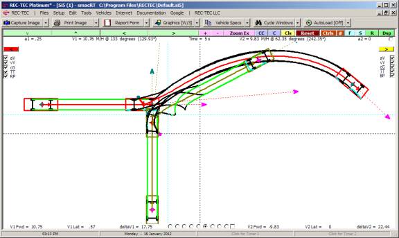
If enough data is available for both the reconstruction and the subsequent SMAC simulations, the results of the SMAC-RT run should match the scene evidence, including the tire traces and the damage to the vehicles resulting from the collision.

New Procedures and Protocols in SMAC-RT:

(Table of Contents)

REC-TEC is capable of transferring information from 360 Linear Momentum to SMAC. Without vehicle information, only very basic information can be transferred. REC-TEC Platinum can compute the Centroid of Damage for the vehicles if CRUSHV information (.crs file) is introduced into the 360LM module (see Animation interface). The program also computes the Kv values for both of the vehicles. The help file for 360 LM contains additional information on this topic.

In REC-TEC Platinum, SMAC-RT incorporates a Collision Interface Protocol (CIP) that will reposition the point of collision interface on the display with or without a bitmap file in place.

Open the SMAC-RT module in REC-TEC and “Open” the “LMTransfer.si5” file. “Run” the SMAC simulation. Click on the “Animation” button bringing up the following display.

Figure 566

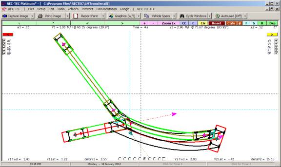
The program drew the animation positioning it in the center of the screen as it automatically engaged the “Zoom Extents” feature prior to setting the configuration for displaying the animation on the screen.

Notice that in the upper right corner of the display is a small round white (radio) button. This button is used to engage or “trigger” the Collision Interface Protocol.

The CIP consists of two steps:

1. Left Click on the current Collision Interface.
2. Left Click on the desired Collision Interface position on the screen.

If an LMTransfer file is loaded, the Collision Interface is located at the 0,0 position. This allows skipping the first step in the procedure as the program will use the 0,0 point as the Collision Interface.

If a non-LMTransfer file is loaded, the Collision Interface is located at an unknown position. This requires that the Collision Interface position be marked on the screen so the program can compute the Collision Interface.

For non-LMTransfer files, once the Collision Interface Protocol button is clicked, the following messages will appear.

Figure 567

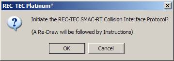
Figure 568

Once the above steps have been completed for non-LMTransfer files, or if the file is an LMTransfer file, the following message will appear.

Figure 569

Place the Cursor on the desired location for the Collision Interface and Left Click on the Mouse. The Animation is automatically redrawn running over your cursor at collision.

You may still draw on the screen using the mouse. Zooming in and out on the animation or using the “C” or “CC” buttons to alter the animation has no effect on CIP operations.

The Repeat and Display options function differently if a Bitmap is in the scene background. With the bitmap loaded into the module, the program is not allowed to change the position, rotate the diagram (the bitmap cannot be rotated), or independently alter the position of the Collision Interface as it is allowed to do if no bitmap is loaded.

Utilizing the 360LM Transfer with the vehicles from CRUSH in conjunction with the Collision Interface Protocol in SMAC makes the tedious job of positioning vehicles correctly in SMAC and then on a bitmap with the Animation run as an overlay, just a few mouse clicks away. The picture on the next page shows a collision positioned on a Google Earth bitmap with the collision quickly moved to show the Collision Interface at the correct location on the bitmap.

Just because it is easy and quick, it does not relieve the investigator from gathering the information, analyzing it in light of all the facts of the case, and doing a proper reconstruction. These tools in REC-TEC are designed to provide for rapid checking of the hypothesis drawn from the reconstruction. They are not a substitute for the hard work required as an integral part of a good reconstruction.

Figure 570

The image above used a Google Earth captured image that was placed into Microsoft Paint and exported as a JPEG (.JPG) file imported as a bitmap type (.bmp, .gif, .jpg) file. The animation was reduced in size to match the image and positioned using the procedure outlined above. The entire process took less than 10 minutes.

Bitmaps cannot be manipulated in REC-TEC. They must be set up in other programs (CAD or Paint) and turned into a .gif, .jpg, or .bmp file, which can be imported into REC-TEC.

The animation can be manipulated. It can be rotated by 90 degrees at a time. I can be zoomed in or out so that it matches the scale of the bitmap.

Photomaps (Google Earth or Microsoft Virtual Earth) can be rotated and cropped to produce a bitmap that can serve as a background for the animation with or without a CAD overlay for a hybrid-view bitmap. Using the Zoom (+/-) feature, the user can manually attempt to scale the animation to the bitmap.

A more accurate method is to “measure” some features, which then can be used to scale the animation to the bitmap. This feature is only available when a bitmap is loaded. The control for scaling is the radio button located in the upper left of the picture.

Figure 571

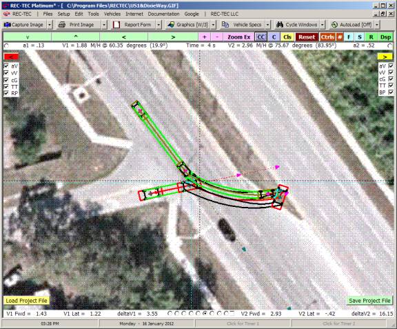
Figure 571 B

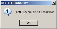
Clicking on the left radio button brings up the above message box. Select two points where the distance between them is known (measured). For this exercise we will use the lane width (distance between lane stripes) with a known distance of 8 feet (96 inches).

Figure 572

After clicking on the second point, an input box appears on the screen asking for the distance between points in inches or millimeters depending on the configuration. After entering the distance, click on OK. This causes a redraw of the animation, which is now scaled to the bitmap.

Figure 573

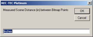
The rescaled animation now must be placed at the correct location over the photograph using the Collision Interface Protocols as outlined above.

Figure 574

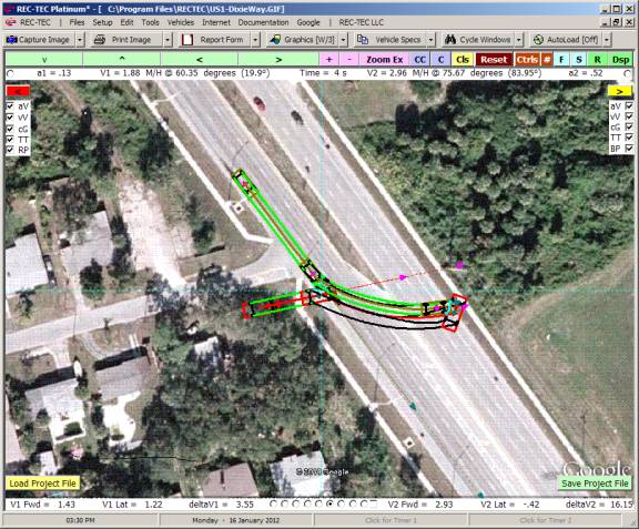
Figure 574 B

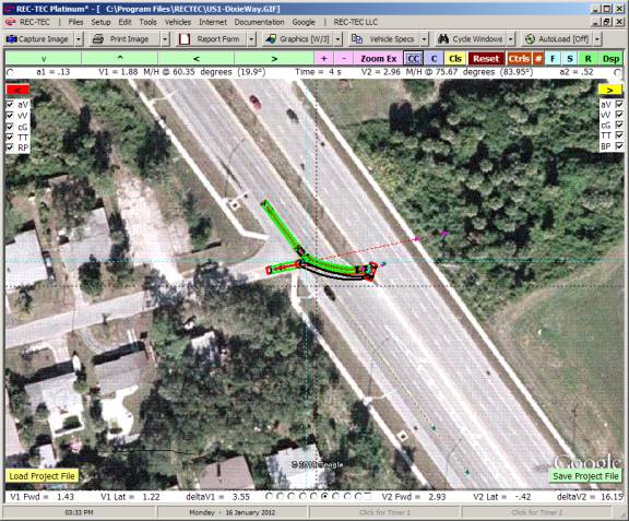
Figure 575 shows the animation scaled to a bitmap, cropped using Paint, and positioned in the correct location using the Collision Interface Protocol. The CTRL button has been used to clear the screen controls.

Figure 575

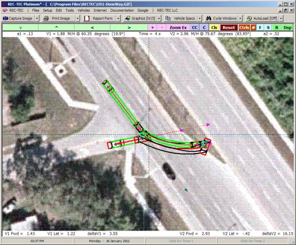
Module 56: Pole / Narrow Object Impact

(Table of Contents) (Table of Contents)

Overview: Computes information for Pole / Narrow Object Impact using Crush/Crash3, Vomhof, Nystrom & Kost, and Wood methodologies.

At the REC-TEC pull down menu, select Energy > Pole / Narrow Object Impact and the Pole / Narrow Object Impact screen appears (Figure 576).

Figure 576

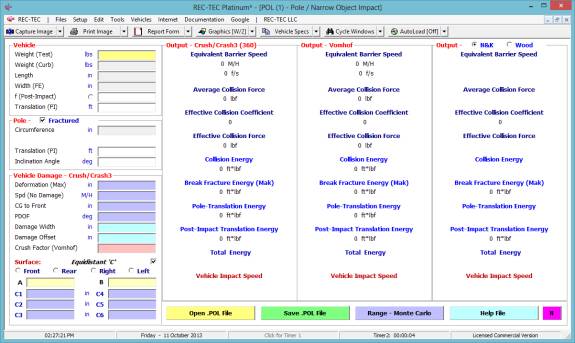
Required Input Data

Vehicle

· Weight (Test) – Weight of Test Vehicle

· Weight (Curb) – Curb Weight of Vehicle

· Length – Length of Vehicle

· Width (FE) – Width of Vehicle (Front End)

· f (Post Impact) – f for Post-Impact Translational Movement

Enter Zero to use Alternate Energy

· Translation (PI) – Distance of Post Impact Translation (Vehicle)

Alternate: Alternate Energy – Post Impact Alternate (Linear and Rotational) Energy

Pole – [Checkbox] – Check if Fractured

· Circumference – Circumference of Pole

Or

· Alternate Energy – Alternate Pole Damage Energy

· Translation (PI) – Distance of Post Impact Translation (Pole)

Enter Zero to denote no translation

· Inclination Angle – Change of Angle resulting from Impact

Vehicle Damage – Crush/Crash3

· Deformation (Max) – Maximum Deformation (Vehicle)

· Spd (No Damage) – No Damage Speed for Vehicle

· CG to Front – Distance from CG to Front of Vehicle (Crash3)

· PDOF – 0 to +/- 180 Degrees: Front = 0 Rear = 180 Left = - 90 Right = 90 (Crash3)

· Damage Width – Width of Damage (Crash3)

· Damage Offset – Measured from CG (Crash3)

· Crush Factor– Vomhof Only

Surface: (Crush/Crash3)

· Front (Front)

· Rear (Rear)

· Right (Right)

· Left (Left)

Equidistant ‘C’ Checkbox[ ] – Check this box for equidistant spaced “C” measurements

· A – “A” Stiffness coefficient

· B – “B” Stiffness coefficient

· C(1-6) – “C” measurements (2 minimum)

· L(1-6) – “L” measurements – L1 is always Zero (0).

Example 1:

Weight (Test) = 3400 lbs

Weight (Curb) = 3388 lbs

Length = 165 in

Width (FE) = 63 in

f (Post Impact) = 0.4

Translation (PI) = 16.8

Circumference = 30.5 in

Translation (PI) = 4 ft

Inclination Angle = 0.71

Deformation (Max) = 20.5 in

Speed (No Damage) = 5 M/H

CG to Front = 74 in

PDOF = 0 degrees

Damage Width = 61.5 in

Damage Offset = 0 in

Crush Factor = 21

Surface: (Crush/Crash3) = Front Equidistant ‘C’ [Checked]

A = 418.4 B = 161.9

C1 = 0 C4 = 13.5

C2 = 5.75 C5 = 1.25

C3 = 11.25 C6 = 0

Figure 577

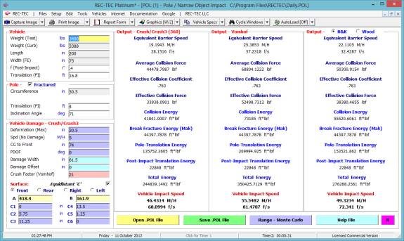
Figure 577 displays the results with the Nystrom and Kost methodology shown in the rightmost panel, while Figure 578 shows the Wood methodology in the rightmost panel.

Figure 578

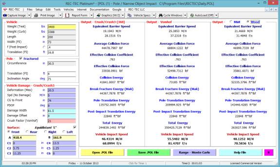
Using the data configuration in Figure 578, Click on the Range – Monte Carlo button to bring up the screen shown in Figure 579.

Figure 579

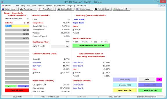
Figures 579 and 580 show the Statistical Range (Monte Carlo) module with the Impact Speed data from the Pole / Narrow Object Impact module. Figure 580 shows the results of a 10K Monte Carlo run.

Figure 580

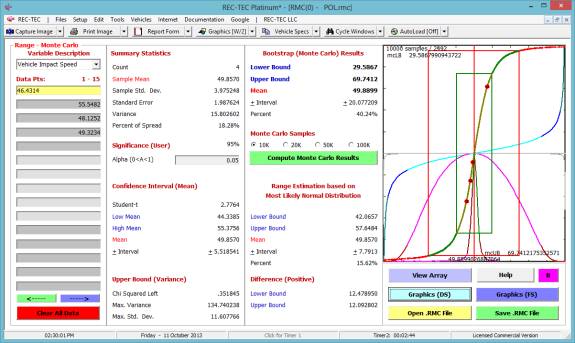
Example 2: Use data from Example 1, but change “C” measurements to non-equidistant with the following values and “L” measurements:

C1 = 0 C4 = 20.5 L3 = 13

C2 = 1.75 L2 = 10 C5 = 1.25 L3 = 15

C3 = 5.25 L3 = 15 C6 = 0 L3 = 10

Figure 581

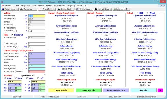
Figure 581 Shows Nystrom and Kost. Figure 582 shows Wood. The only values changed are those in the third output panel (Crush/Crash3).

Figure 582

Setting the Damage width to 0 (zero) effectively removes the Crash3 Vehicle Impact Speed.

Figure 583

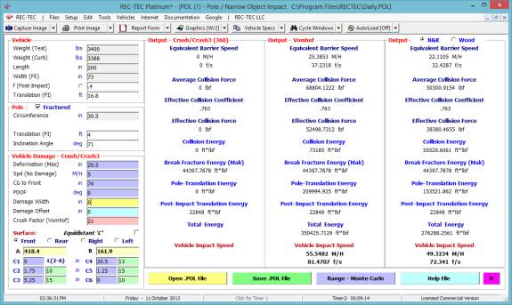
Setting the Deformation (Max) to 0 (zero) effectively removes the Vehicle Impact Speeds from the non-Crash3 methodologies.

Figure 584

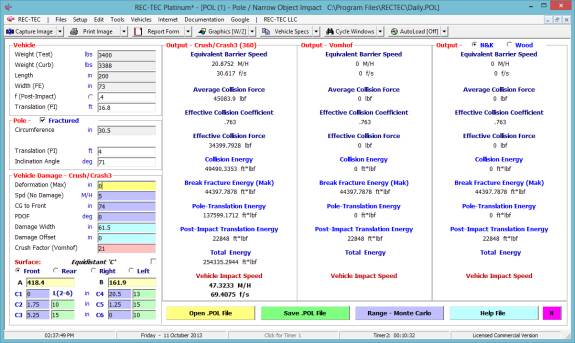
Example 3: Using the non-equidistant values seen in Figure 584, uncheck the “Fractured” checkbox in the Pole frame. Some new poles are labeled with the energy required to “break” the pole. Assume the pole has such a label with 40,000 ft*lbf of energy required to break the pole.

Figure 585

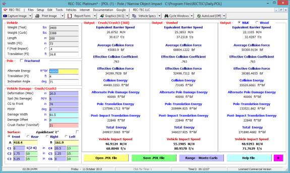
Figure 585 Shows Nystrom and Kost. Figure 586 shows Wood.

Figure 586

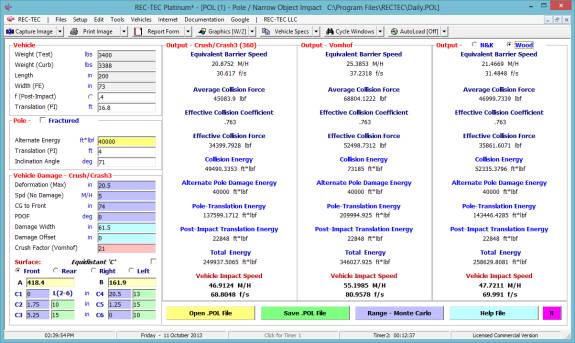
The Vomhof, Nystrom & Kost, and Wood methodologies are designed to handle frontal impacts with the maximum deformation in line with the center of mass of the vehicle. While this may frequently occur in test collisions and suicides, it rarely happens in real-life, pole/narrow object impacts.

The Vomhof methodology can theoretically be used for side impacts, but the modified “Crush Factor” equation (with the CF multiplied by 0.6) has not been tested on side impact collisions with a PDOF that is not perpendicular to the side struck, mandating that the impact must be along the PDOF and in line with the center of mass.

The limitation described does not apply to the Crush/Crash3 methodology. The pole damage can be on any surface of the vehicle, with any PDOF appropriate to the surface struck.

It is very likely that rotation of the vehicle would occur post-impact using the Crush/Crash3 methodology. The energy going into post impact rotation should be considered along with the post-impact translation. This condition can be accommodated by adding the rotation energy and translation energy, and by entering a 0 (zero) for f (Post Impact), enter the computed post-impact energy total as Alternate Energy (PI)

Figure 587

Module 57: Energy – Damage Analysis > Crush (Motorcycle)

(Table of Contents) (Table of Contents)

Overview: Computes Speed from Motorcycle Crush Analysis. The paper “Motorcycle Crush Analysis” (Help Button) is a reprint of the article by Wade Bartlett, PE appearing in Accident Reconstruction Journal in March/April 2009. The paper is used with permission of the author and Vic Craig, Editor of the Accident Reconstruction Journal.

At the REC-TEC pull down menu, select Energy – Damage Analysis > Crush (Motorcycle) and the Crush (Motorcycle) screen appears (Figure 588).

Figure 588

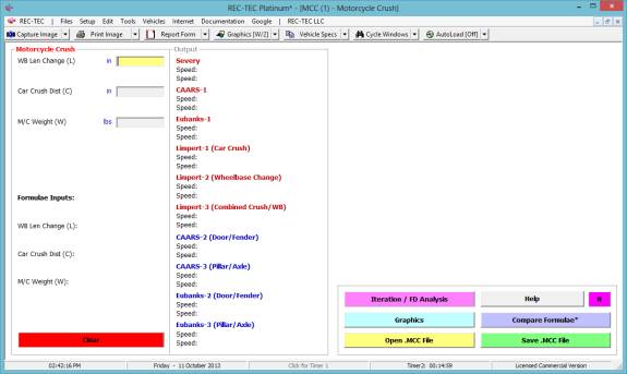
Required Input Data

· WB Len Change (L) – Change in Wheelbase Length

· Car Crush Distance (C) – Car Crush Distance

· M/C Weight (W) – Weight of Motorcycle

Example 1:

WB Len Change (L) = 15 in

Car Crush Distance (C) = 20 in

M/C Weight (W) = 450 pounds

Figure 589

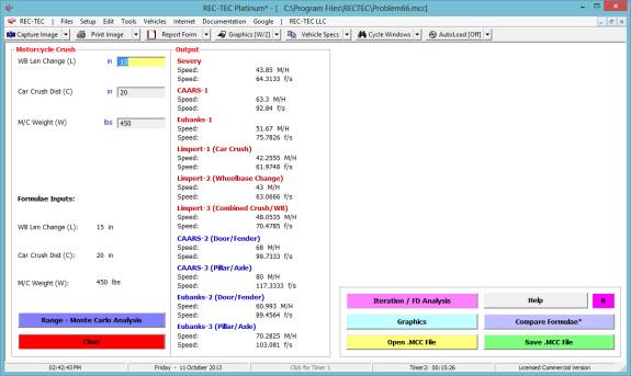
Figure 589 displays the results, while Figure 590 shows the results and the Graphics.

Figure 590

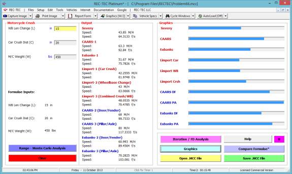
Figure 591 shows the Finite Difference Analysis Menu.

Figure 591

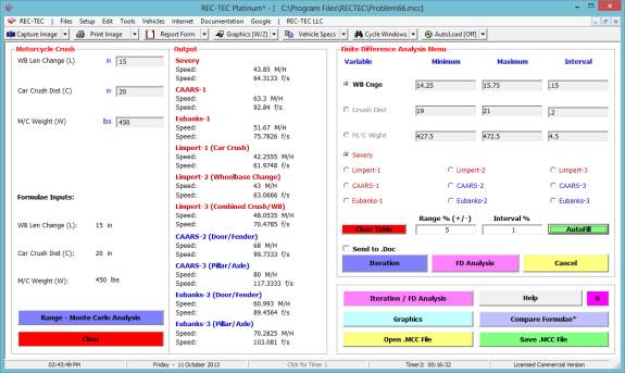
Figure 592 shows the Finite Difference Analysis using the Severy formula.

Figure 592

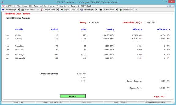
Figure 593 shows the Iteration using the Severy formula.

Figure 593

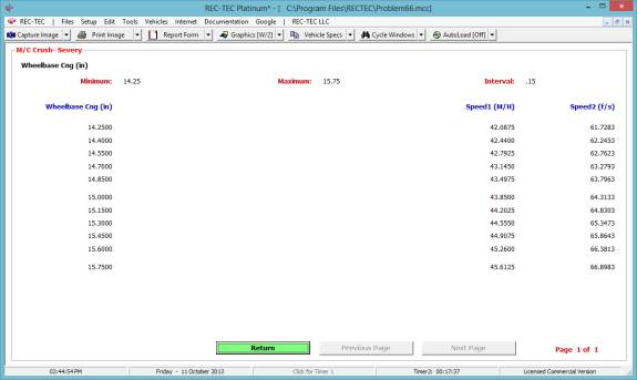
Figure 594A shows the Formulae Comparison.

Figure 594A

Figure 594B shows the Finite Difference Analysis using the CAARS (D/F) formula.

Figure 594B

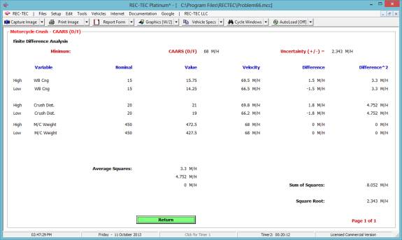
Figure 594C shows the Finite Difference Analysis using the Eubanks (P/A) formula.

Figure 594C

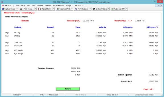
Module 58: Vectors (EDR – Momentum)

(Table of Contents)

Overview: Computes the Resultant vector (Length and Angle) from the Longitudinal and Lateral DeltaV vectors downloaded from Event Data Recorders. With additional inputs it can compute DV1, DV2, V1, V2, V3, and V4.

At the REC-TEC pull down menu, select Vectors (EDR – Momentum) and the EDR – Vectors screen appears (Figure 595).

Figure 595

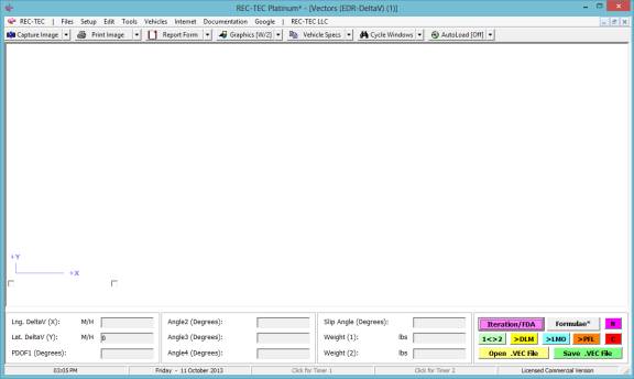
Figure 596

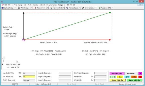
Figure 596 displays the resultant for the data entered. There is no requirement to identify the units for the inputs, as the output will be the same as the input.

Figure 597

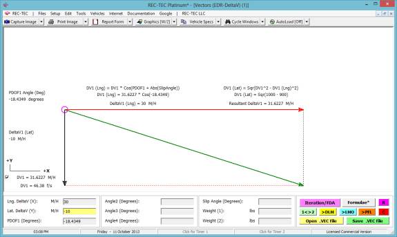
Figure 597 displays the resultant for the data entered when a negative value is entered for the lateral DeltaV. There is no requirement to identify the units for the inputs, as the output will be the same as the input.

Figure 598

Figure 598 displays the resultant for the data entered when a negative value is entered for both the lateral and longitudinal DeltaV. There is no requirement to identify the units for the inputs, as the output will be the same as the input.

Vectors and New Technology

2D Angular Collision Alternative to V3 and V4 Requirement
(Table of Contents)

Four modules in REC-TEC now offer an alternative to requiring V3 and V4 speeds to reach a collision solution.

Digital Momentum, Linear Momentum, PDOF/360LM in the 360 LM mode and Solver Functions > Vector now can use the Longitudinal DeltaV and PDOF for one vehicle (Vehicle 1) to solve for DV1, DV2, V1, V2, V3, and V4. This method uses the Law of Sines, the Law of Cosines and Newton’s Third Law of Motion. In Digital Momentum, Linear Momentum and 360 LM the program solves for V3 and V4 using this method and then uses those values to solve the Conservation of Linear Momentum (COLM) equations. In Solver Functions it uses this method to solve for all of the unknowns.

Longitudinal DeltaV (X) - (CDR download)

Lateral DeltaV (Y) - (CDR download)

or

PDOF1 (Degrees) - User supplied

Angle 2 (Degrees)

Angle 3 (Degrees)

Angle 4 (Degrees)

Slip Angle (Degrees) [Optional] – Angle between the Longitudinal Axis of Vehicle 1 and its Post-Impact direction of travel

Weight (1)

Weight (2)

With Event Data Recorder (EDR) downloads becoming increasingly available, this new methodology offers a valuable alternative to the V3 and V4 requirement, one not always as reliable or accurate as desired. It also offers a convenient cross check when V3 and V4 are available.

Formulae:

DV1 = DV1X / Cos(PDOF1 + Abs(SlipAngle))

DV2 = DV1 * (W1 / W2)

AngleC = 180 - (A3 + PDOF1)

AngleA = A2 - A4

PDOF2 = 180 - (PDOF1 + A2)

AngleB = 180 - (PDOF2 + AngleA)

V1 = DV1 * Sin(AngleC) / Sin(A3)

V3 = DV1 * Sin(PDOF1) / Sin(A3)

V2 = DV2 * Sin(AngleB) / Sin(AngleA)

V4 = DV2 * Sin((180 - (AngleB + AngleA)) / Sin(AngleA)

In Digital Momentum, Linear Momentum and 360 LM, entering an “X” for V3 brings up a display for entering the Longitudinal DeltaV, PDOF and Slip Angle. The other variables should be entered in their regular locations for the particular module.

The Solver Functions > Vector module has entry locations for all of the required variables as long as no entry is made in the Lateral DeltaV input location. It also has a Formulae* button that will display the interactive formulae and variables used in the computations. The vector speed solutions are displayed in Primary and Secondary output modes along with a graphical display of the collision including DeltaV/PDOF vectors.

All of the Examples will use the following data except as noted:

Longitudinal DeltaV = 12.06 M/H

Angle 1 = 0 degrees

Angle 2 = 90 degrees

Angle 3 = 40 degrees

Angle 4 = 25 degrees

PDOF1 = 58 degrees

Slip Angle = 0 degrees

Weight 1 = 3000

Weight 2 = 2000

Example 1 – Digital Momentum

Placing an “X” in the V3 Speed box and entering it brings up the DeltaV Computation Inputs frame.

Figure 599

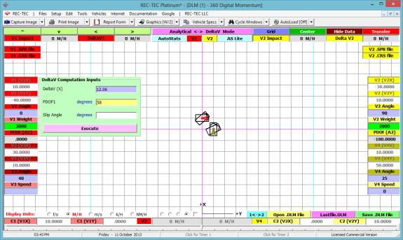
Entering the data and clicking on the Execute button creates Figure 600.

Figure 600

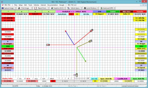
Example 2 – 360 Linear Momentum

Placing an “X” in the V3 Speed box and entering it brings up the DeltaV Computation Inputs frame and hides the V3 and V4 Speed inputs.

Figure 601

Entering the data and clicking on the Execute button creates Figure 602.

Figure 602

Figure 603 shows the Graphics – Right Clicking on the Graphics will bring up various Vector displays.

Figure 603

Example 3 – 360 LM Lite

Placing an “X” in the V3 Speed box and entering it brings up the DeltaV Computation Inputs frame.

Figure 604

Entering the data and clicking on the Execute button creates Figure 605.

Figure 605

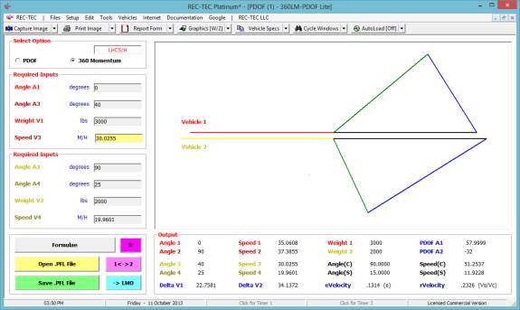
Example 4 – 360 Vectors (EDR-DeltaV)

Note: In late 2011 this module was upgraded and the inputs were changed from those shown in Figures 595-598. The upgraded Vector module is now capable of sending its Momentum solution directly to the 360 Linear Momentum module using the [> LMO] button. Two Check Boxes have also been added in front of the DV1 and DV2 solutions. Placing a check in one of these boxes will bring up the Solution Diagram for the corresponding PDOF/DeltaV. Un-checking the box will return the user to the Momentum Vector diagram. Using the [Esc] key will show the Longitudinal and Lateral components used to arrive at the PDOF solution if that methodology was employed in the solution. The ToolTips (place cursor over the inputs or Check boxes) will describe the effect these actions will have on the modules displays. Figures 606-609 have been upgraded and additional Figures have been added.

Right clicking on Formulae* after entering the data results in Figure 606.

Figure 606

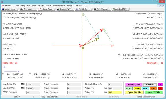
Figure 607 uses an 80-degree approach angle for Vehicle 2.

Figure 607

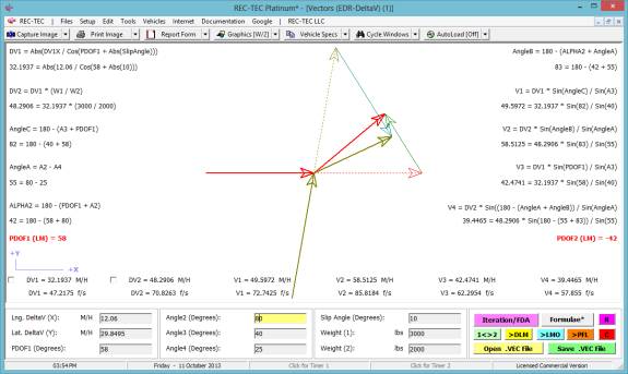
Figure 607 uses 80 degrees for Angle 2

Figure 608 uses a 100-degree approach angle for Vehicle 2.

Figure 608

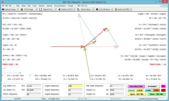
Figure 608 uses 100 degrees for Angle 2

Figure 609 uses a 10-degree Slip Angle to calculate DV1 with Angle 2 back at 90 degrees.

Figure 609

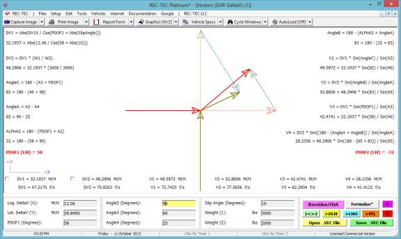
Figure 609 uses a 10-degree Slip Angle to calculate DV1 with Angle 2 back at 90 degrees and with a Lateral DeltaV used to compute the PDOF angle of 58 degrees.

Figure 610

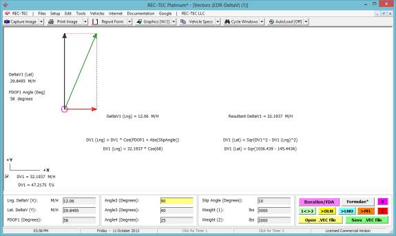
Figure 610 shows the DV1 Vector Diagram with a Check in the DV1 Checkbox. The screen shows a PDOF1 of 58 degrees along with the 10-degree slip angle used in the computations. The [Esc] key brings up the data for the initial computation of 58 degrees based on the Lateral Input and does not account for the Slip angle (Figure 611).

Figure 611

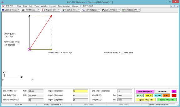
A second [Esc] key returns the screen to the initial Momentum diagram (Figure 612).

Figure 612

Major Upgrade

In July of 2014, this section underwent a major upgrade and a name change to Vectors (EDR-Momentum), more accurately reflecting the capabilities of the module.

Figure 612-U1

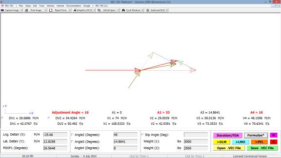
If using the AutoLoad feature when the module is first called up after the version upgrade, the only noticeable changes are:

1. The name change for the Module
2. New blocks appear over the DV2, V1, V2, V3, and V4 solution blocks
1. Adjustment Angle
2. A1 = 0
3. A2 = 55
4. A3 = 14.8641
5. A4 = 10
3. Checkboxes are now in front of Angle2, Angle3 and Slip Angle
4. The 1<>2 button is no more.

The tour of the new features in the upgrade will start with Clicking on the Formulae* button.

Figure 612-U2

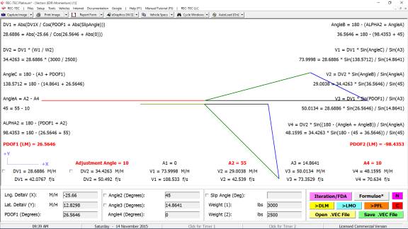
At first it may look like the Graphics have been messed up. This is just the Graphics configuration for the LM-PDOF Lite module shown on the Vector screen. Right clicking the mouse will restore the more familiar 360 LM configuration.

Figure 612-U3

Time to show where the Adjustment Angle comes from. Notice the Checkbox in front of Slip Angle? Click on it and Slip Angle changes to Adjustment Angle and you will notice it is set to 10. Notice that it has changed the base angles (below the Graphics Screen) to the Angles shown in red on the Graphics screen. We will come back to this later as it is a Major feature critical to the accuracy of the rest of the upgrades.

Figure 612-U4

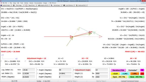
Notice that there is a Checkbox in front of the Angle2 input line below the Graphics.

Figure 612-U5

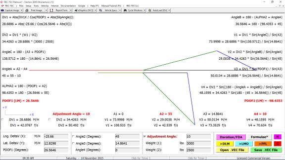
Clicking on that Checkbox brings up an Input for the V1 speed which should show 74 M/H if that is the Primary input. A keen eye will notice that some of the Formulae have changed along with the data. The Input block asking for Angle3 has disappeared but the Checkbox remains. The Angle4 input has changed to "Angle Change (A2 to A4)" and now shows 45 instead of 0. Note also that in the Formulae on the Graphics screen, V1 is described as an Input of 74.

The Adjustment Angle now shows "N/A" as angles are not required to perform these computations so there are no angles to adjust. Angles A2, A3, and A4 are computed by the program and inserted into the respective Angle Inputs for future analysis. The Angles shown on the Graphics screen do not include the Angle Adjustment.

Notice again the Checkbox in front of where the Angle2 input line was below the Graphics. Right click on it.

Figure 612-U6

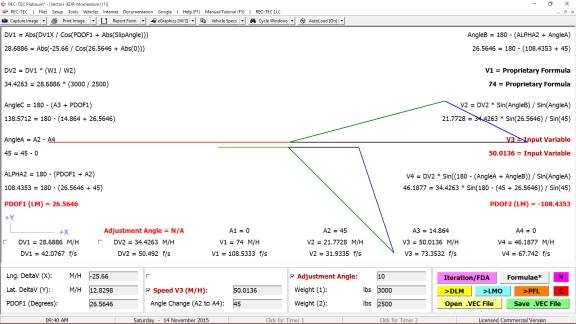
Clicking on that Checkbox brings up an Input for the V3 speed, which should show 50.0136 M/H if that is the Primary input. A keen eye will notice that some of the Formulae have again changed along with the data. The Input block asking for Angle2 has disappeared but the Checkbox remains. The Angle4 input still shows the change to "Angle Change (A2 to A4)" and still shows 45 instead of 0. Note also that in the Formulae on the Graphics screen, V3 is described as an Input of 50.0136. Notice that V1 now shows 73.9999 (truncation) and Proprietary Formula. The specific formula is not needed as it can be proved correct using a variety of methods.

So How did we get V3 and Why? Tackling the "Why" question first, because maybe the EDR did not collect the V1 information and we were unsure of other methods of obtaining V1. If we are able to get a good post-impact speed at separation for V3, it is always a good idea to run it as a cross check. Why not bolster your own case whenever possible? As for the "How" aspect, one good way is to do a skid to stop computation if possible, but this is just one of many ways that may present themselves.

The Adjustment Angle now shows "N/A" as angles are not required to perform these computations therefore there are no angles to adjust. Angles A2, A3, and A4 are computed by the program and inserted into the respective Angle Inputs for future analysis. The Angles shown on the Graphics screen do not include the Angle Adjustment.

Care to guess what happens when we uncheck the V3 Checkbox?

Figure 612-U7

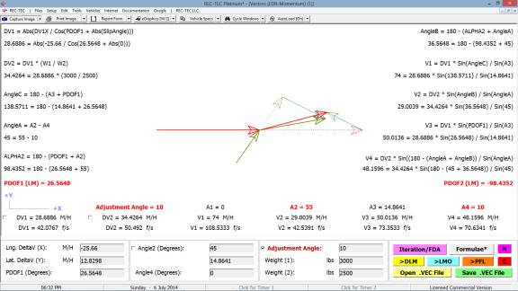
Time to play with the Adjustment Angle. Change it to Zero.

Figure 612-U8

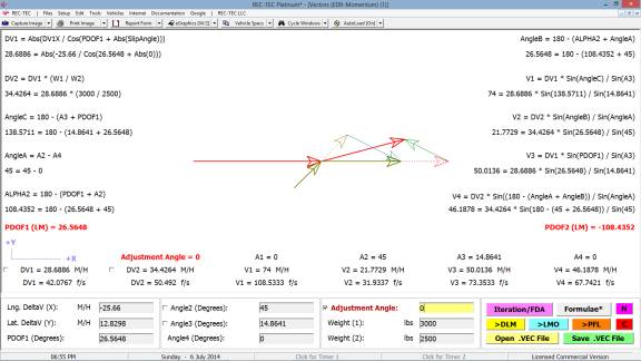
Notice that the Angles on the Graphics section have changed. Look what also changed; V2 and V4. Note that V1 and V3 have not changed. As long as we are playing with the Adjustment Angle, why not make it 30?

Figure 612-U9

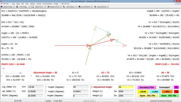
Hmmm? Is that OK? It is inside of the Cone of Departure. It looks like the centers of mass have crossed. What if we send this to 360 Linear Momentum and see what happens? Left click on the light blue >LMO button.

Figure 612-U10

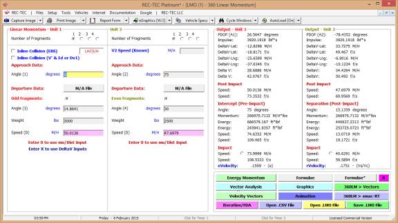
It looks like the same problem and we are getting the same answers.

Figure 612-U11

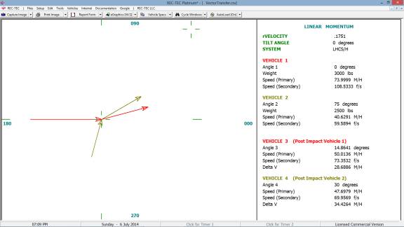
Graphics look OK. Let's give Vector Sum Analysis a go at it.

Figure 612-U12

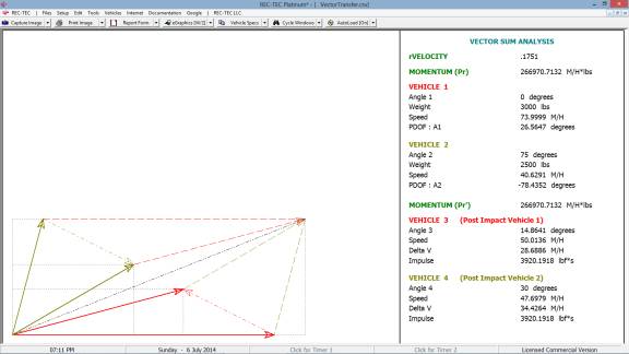
Everything seems to be just fine here too. Looks like we have a winner. Before getting too cocky, lets go back to the Vector Screen, and select the V1 Speed Checkbox.

Figure 612-U13

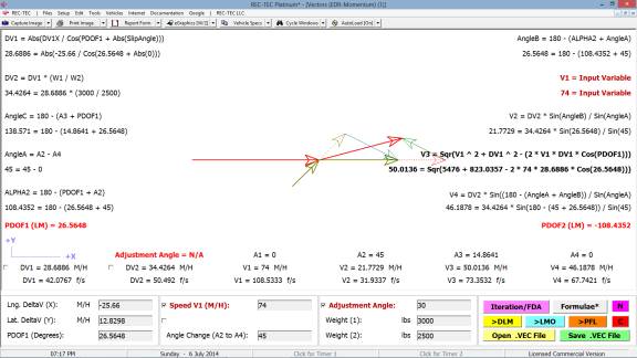
The numbers are back to the original numbers for the V1 Speed Input. Transfer this to 360 Linear Momentum.

Figure 612-U14

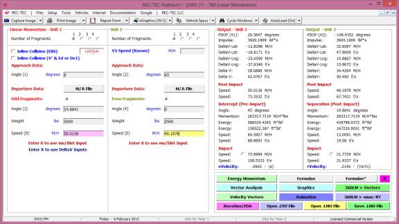
The problem and answers appear to be the same as on the Vector screen. Go to Graphics.

Figure 612-U15

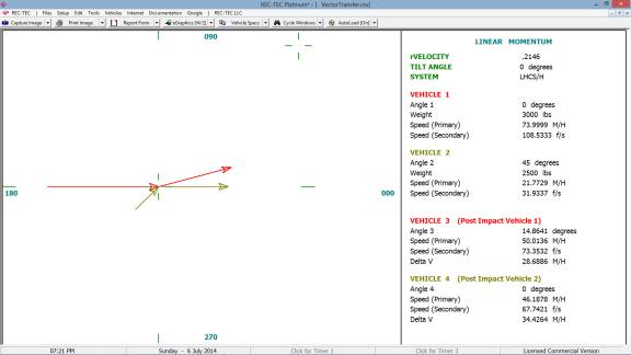
That looks OK. Now go to Vector Sum Analysis.

Figure 612-U16

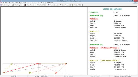
Looks different than Figure 612-U12, but both resultant vectors overlap each other and they meet at the same point. It must be OK.

How can they both be OK and be so different? It is because the answers are different. Look at the V2 and V4 speeds in both problems. They are very different.

So what is the point?

The point is there is more than one solution that is mathematically correct, but there is only one solution that matches what actually happened. While the speed differences for Vehicle 2 at impact were minimal in these two problems, let's look at one more scenario.

Change the Adjustment Angle to 45.

Figure 612-U17

Figure 612-U18

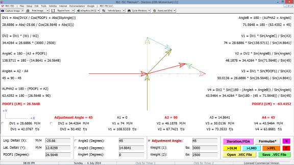
Figure 612-U19

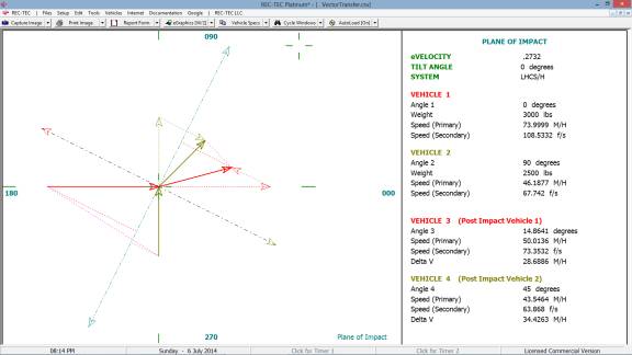
Figure 612-U20

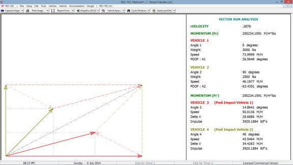
V2 has gone from 21 M/H to over 46 M/H. That could certainly be enough to make a huge difference, both in a Civil venue and in a Criminal one.

That is the point!

Module 58B: Vectors (Inline Momentum)

(Table of Contents)

Overview: Computes collision information including Impact and Post-Impact speeds, closing and separation speeds, and DeltaV data for both vehicles based on Event Data Recorded outputs from only one vehicle if the weight of the other vehicle is known.

At the REC-TEC pull down menu, select Vectors (EDR) > Vectors (Inline Momentum) and the Vectors - Inline Momentum screen appears (Figure 612-IM1).

Figure 612-IM1

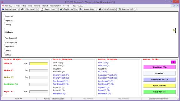
Required Inputs:

• Delta V1 – EDR data
• Weight V1 – Weight of Vehicle 1
• Weight V2 – Weight of Vehicle 2
• Restitution (e) – Determined by reconstructionist
• Impact Speed V1 – EDR data

This module is limited to Inline Collisions. While it requires very few inputs, it can produce an exceptional amount of data. The "Restitution (e)" input is critical and the utmost care should be exercised in the determination of this value. The range for this value in both Finite Difference Analysis and Iteration should be carefully thought out, not just haphazardly entered as it is critical in the computations.

Output:

The output from this module consists of the repeated Input variables (shown in black in the Output frames) plus the Unknowns (shown in blue in the Output frames) expressed in the Primary and Secondary configurations as selected in the Setup > REC-TEC menu. These Outputs consist of:

• Delta V2 (second vehicle in collision)
• Closing Velocity (Vc)
• Separation Velocity (Vs)
• Impact (V2)
• Post-Impact V1 (V3)
• Post-Impact V2 (V4)

Example 1: The EDR gives a DeltaV of 30 M/H with an Impact speed of 47.5 M/H. It was estimated that the restitution value was .2. The weight of Vehicle 1 was 4000 and the weight of vehicle 2 was 3000.

Figure 612-IM2

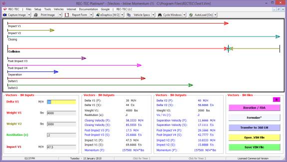
The inputs have determined that this was a head-on collision and have yielded a complete collision profile from very limited data. Figure 612-IM3 shows the primary Formulae.

Figure 612-IM3

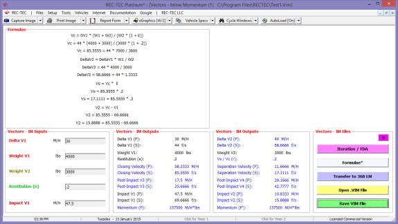
Figure 612-IM4

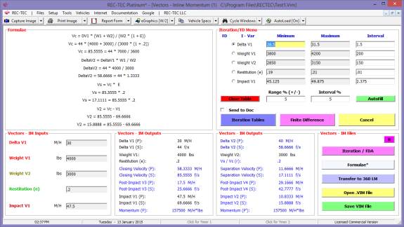
Clicking on Iteration/FDA brings up the control interface for Iteration and Finite Difference Analysis. Entering 5% for both Range and Interval sets up the Minimum and Maximum values shown in Figure 612-IM4.

Figure 612-IM5

Figure 612-IM5 shows Interval adjustments made to the Delta V1 and Restitution values. These adjustments will be used in the Iteration and FDA screens shown below.

Figure 612-IM6

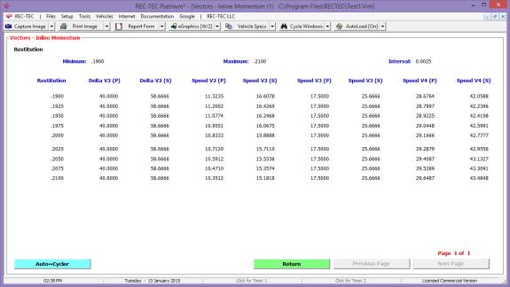
Restitution iteration shown above.

Figure 612-IM7

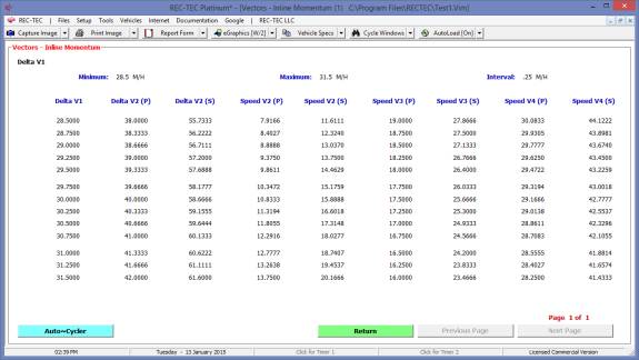
Delta V1 iteration shown above.

Figure 612-IM8

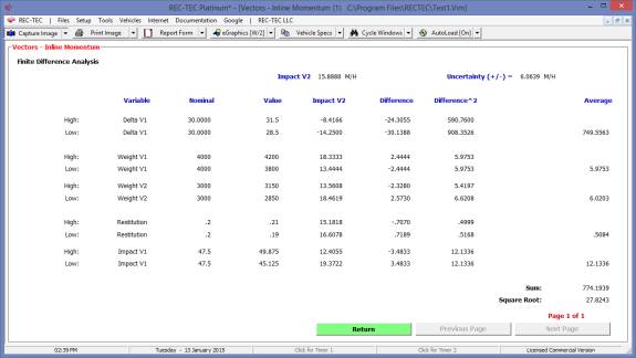
Figure 612-IM8 (shown above) shows the FDA Uncertainty value of +/- 6.0639 M/H for the Impact Velocity of Vehicle 2. The very high sensitivity to changes in Delta V1 values is clearly demonstrated by the high values shown for this variable.

Figure 612-IM9

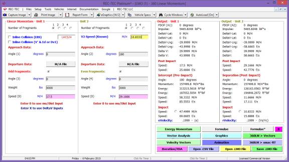
Figure 612-IM9 shows the same problem automatically transferred into 360 Linear Momentum. The answers differ in the 4th decimal place. This serves as an excellent cross check on the accuracy of the values computed using the Vectors (Inline Momentum) module.

Example 2: The EDR gives a DeltaV of 40 M/H with an Impact speed of 10.8333 M/H. It was estimated that the restitution value was .2. The weight of Vehicle 1 was 3000 and the weight of vehicle 2 was 4000. This results in a head-on collision. This example is the reverse of Example 1.

Figure 612-IM10

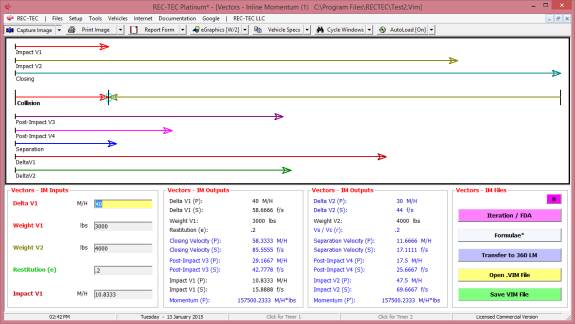
Figure 612-IM11

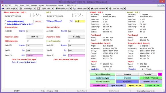
The Example 2 problem transferred into 360 Linear Momentum is shown in Figure 612-IM11.

Example 3: Same as Example 2 but with a restitution(e) value of Zero (0).

Figure 612-IM12

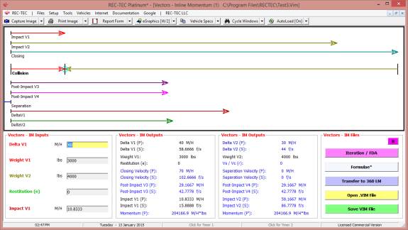
Figure 612-IM13

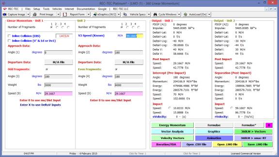
The Example 3 problem transferred into 360 Linear Momentum is shown in Figure 612-IM13.

Example 4: The EDR gives a DeltaV of 10 M/H with an Impact speed of 20 M/H. It was estimated that the restitution value was .3. The weight of Vehicle 1 was 3000 and the weight of vehicle 2 was 2000. This results in a rear-end collision.

Figure 612-IM14

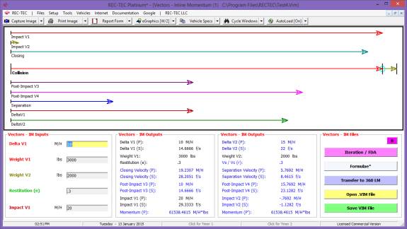
Figure 612-IM15

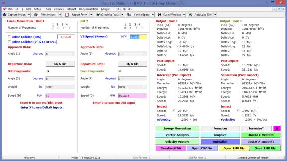
The Example 4 problem transferred into 360 Linear Momentum is shown in Figure 612-IM15.

Example 5: The EDR gives a DeltaV of 30 M/H with an Impact speed of 30 M/H. The restitution value is Zero (0). The weight of Vehicle 1 is 3000 and the weight of vehicle 2 is 3000. This results in a head on collision.

Figure 612-IM16

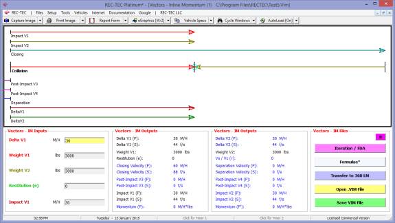
Figure 612-IM17

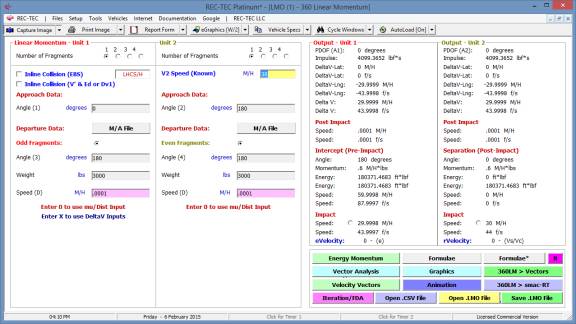
The Example 5 problem transferred into 360 Linear Momentum is shown in Figure 612-IM17.

Module 59: Collision Avoidance > Separation Distance

(Table of Contents) (Table of Contents)

Overview: Computes minimum separation distance between vehicles necessary for the Following Vehicle to react and stop with the required distance between vehicles when both have come to a full stop.

At the REC-TEC pull down menu, select Collision Avoidance > Separation Distance and the Collision Avoidance – Separation Distance screen appears (Figure 613).

Figure 613

Required Inputs:

• ‘g’ Deceleration (Vehicle 2 - Target) – Corrected for grade and braking
• Speed (Initial) – V2 Initial Speed
• ‘g’ Deceleration (Vehicle 1 - Bullet) – Corrected for grade and braking
• Speed (Initial) – V1 Initial Speed
• Reaction Time – Reaction Time for V1
• Distance (Safe) – Desired Safe Distance between vehicles when both have reached full stop

Example 1: Vehicle 2 is at 20 M/H and Vehicle 1 is at 30 M/H when Vehicle 2 begins a maximum rate deceleration. The Reaction Time for Vehicle is 1 second to begin a maximum rate deceleration. Both vehicles decelerate at .7 ’g’ to a full stop. The desired Safe distance between vehicles is 15 feet.

Figure 614

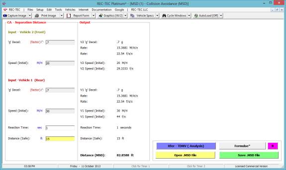
Figure 615 (with Formulae)

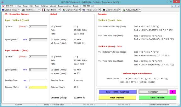
Figure 616

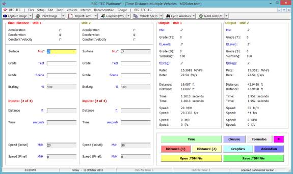
Figure 616 shows the data transferred to the Time Distance Multiple Vehicle Module. The transfer has automatically set up the Animation in this module as seen in Figure 617.

Figure 617

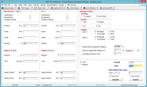
Clicking on the Execute button creates the Animation shown at completion in Figure 618.

Figure 618

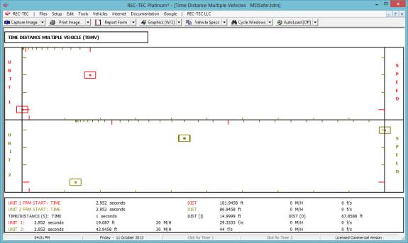
Note that the “DIST (I)” or Instantaneous Distance at Stop is 14.9999 ft.

Module 66: Traffic Engineering – School Bus Stop

(Table of Contents)

Traffic Engineering – School Bus Stop

Overview: Displays graphically the specifications of a school bus stop.

Entry into Module:

At the REC-TEC pull down menu, select Traffic Engineering > School Bus Stop and the Traffic Engineering block and click on School Bus Stop screen appears (Figure 619).

Figure 619

Entering a Roadway Speed (Signed speed of Roadway + 5 miles per hour) causes the Graphics screen to appear (Figure 620).

Figure 620

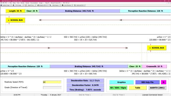
Figure 620 has the Upper section of the display with a school bus being approached from the rear. Color-coded blocks above show the required Clear Distance (25 ft), the computed Braking Distance based on a deceleration rate of 11.2 f/s/s, and the distance covered in the required 2.5 second Perception Reaction Time. Notice in the Menu Bar that for eGraphics, the selected configuration is a White background with a #2 line width.

Figure 621

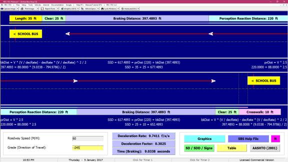
Figure 621 has the Lower section of the display with a school bus being approached from the front. Color-coded blocks below show the Crosswalk (10 ft), the required Clear Distance (25 ft), the computed Braking Distance based on a deceleration rate of 9.7411 f/s/s (adjusted for Grade), and the distance covered in the required 2.5 second Perception Reaction Time. Notice in the Menu Bar that for eGraphics, the selected configuration is now a Blue background with a #5 line width as selected by the user.

The inter-active formulae for the front/rear approaches are shown directly below each approach. The inter-active computed Deceleration rate (adjusted for Grade), the corresponding Deceleration Factor, and the Braking Time are each shown in the lower center of the screen.

While the ability to draw on the Graphics screens in REC-TEC has not changed, for 2017 we have changed the color from light gray on the screens to Black if the screen is in White background and White if the screen is in Blue (or an alternate background color). Left clicking on Graphics or Reset, and right clicking on the graphics will clear the screen of any drawing while forcing a redraw of the screen.

Clicking on SSB Help brings up a 4-page IOWADOT Office of Traffic and Safety document dealing with School Bus Stops. The scenario from this document is used for the problem shown in this section.

Clicking Table shows a single-page based on the input information for Speed and Grade (Figure 622).

Figure 622

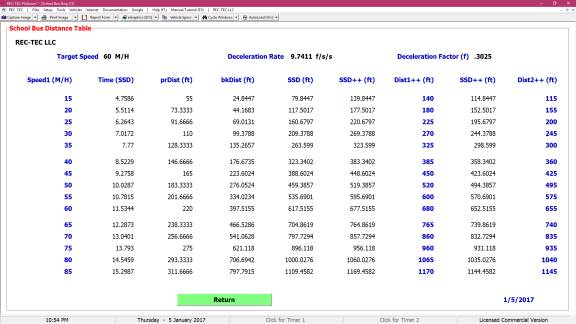
In addition to the [F1] key onboard Help file, the [F5] key Inside REC-TEC manual and tutorial and the 2001 AASHTO manual (.pdf) are available from our website.

The SD / SSD / Signs button will bring up guidelines for Stopping Distance, Stopping Sight Distance, and requirements for School Bus Stop Signs.

Module 67: Traffic Engineering – Work Zone (MUTCD)

(Table of Contents)

Traffic Engineering – Work Zone (MUTCD)

Overview: Displays graphically the specifications of a Work Zone (MUTCD).

Entry into Module:

At the REC-TEC pull down menu, select Traffic Engineering > Work Zone (MUTCD) and the Traffic Engineering block and click on Work Zone (MUTCD) screen appears (Figure 623).

Figure 623

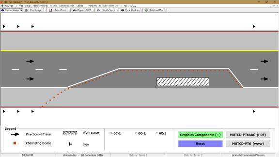
The Module opens with the above screen (Figure 623) displaying the first of three basic displays from the MUTCD Chapter 6C.

This display shows the Legend to help with understanding the different elements in the diagram. Clicking on the Graphics Components button will create Figure 624 numbering various sections of the diagram and allowing ToolTips to identify and describe these components using the correct nomenclature.

Figure 624

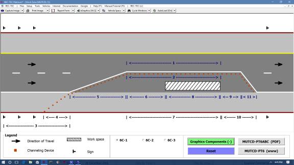
Selecting the center option in the lower center frame (6C-2) creates Figure 625

Figure 625

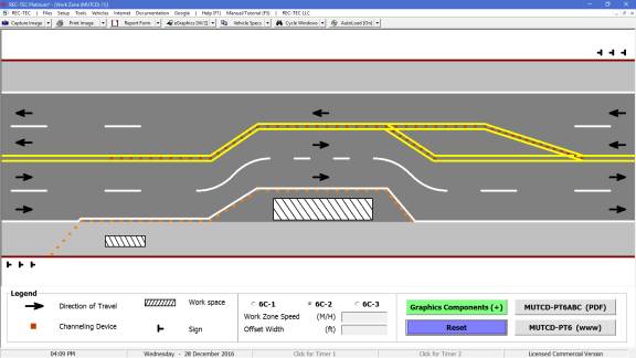
The lower center frame for this selection adds 2 inputs, Work Zone Speed and Offset Width. These will allow computation of distances for some of the elements in the diagram, shown in red in Figure 626 when values for both inputs have been entered and the Graphics Components button is clicked.

Figure 626

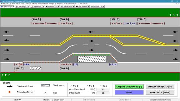
This screen got very colorful. Notice that the eGraphics on the lower Menu Bar shows B/2 denoting that color has been added to the diagram for use with a computer screen or for printing in color. It also shows measurements (corresponding to the speed and offset values entered) above or below a particular element.

Figure 627

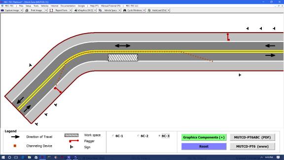
Diagram 6C-3 (Figure 627) is back to the white background without the added graphics components. It does have something added to it that the other two did not have, a Flagger symbol in the Legend and in the diagram.

Clicking on the Graphics Components button brings up Figure 628 with its colorful background and a much larger Channeling Device thanks to an increase in Line width in eGraphics.

Figure 628

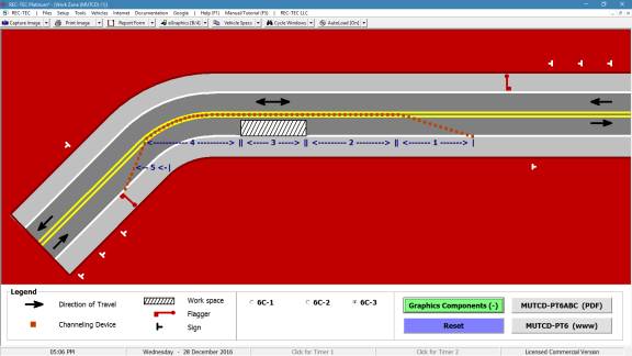
The ability to toggle the Graphics Components may help users to learn the various element names and descriptions depicted in the 3 basic Temporary Work Zone displays. It will permit self-testing with answers immediately available in the ToolTip (not shown here). It offers a choice.

Now for a few disclaimers:

1. This is not a substitute for an engineering study.
2. The computations are speed dependent.
3. The distances resulting from these speeds are suggested minimums.
4. Check Your State – Many states have there own rules.
5. Please – Read the Manual (MUTCD).

Module 68: DrawPad

(Table of Contents)

Overview: Module allows simple drawings to be created, manipulated, and turned into Bitmap (.bmp) files. Pre-existing BMP, JPG, and GIF files can be imported, modified, and saved as .BMP files.

Entry into Module:

The DrawPad link is on the REC-TEC Main Interface Menu line next to the License Name. Click to Initiate DrawPad (Figure DP1).

Figure DP1

Figures DP1 and DP2 show two different color palettes, available for Draw and Background. The menu at the bottom of the screen shows the various items with the Radio Buttons used to make the selection. Each of the items and their radio buttons all have Tool tips describing their functions.

Figure DP2

Images (discussed later) can be imported (Figure DP3). An Image can be Cropped, Moved, Rotated, and Drawn upon.

Figure DP3

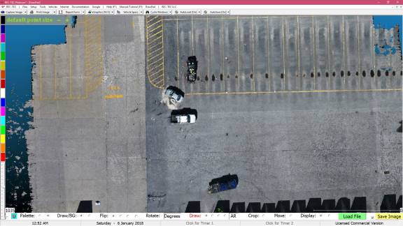
Figure DP4

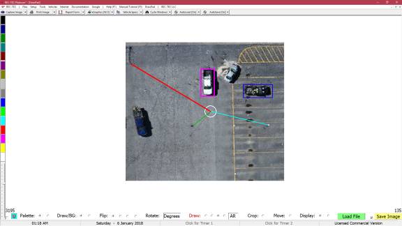
Intermediate steps can be saved as an Image, retaining any lines drawn on the Bitmap file, which becomes Picture1 when loaded. This allows the user to “Undo” the last object drawn using the small Undo Button (light blue with a red U in the center – lower left of the screen). Just to the left is a small white Checkbox used to switch the cursor between a crosshair and a spinning blue circle that may be easier to use against some backgrounds. On the left of the Checkbox is the Slider used to Scale (Up or Down) the bitmap maintaining the original Aspect Ratio. If additional scaling is needed, save the image and then reload it to rescale even further.

Figure DP5

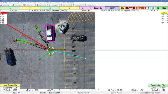
Figure DP5 shows a SMAC collision being run over the bitmap in Figure DP4. SMAC can be scaled to the Bitmap created in DrawPad (see smacRT discussion - Table of Contents>Module 55 or here http://www.rec-tec.com/Inside_REC-TEC.htm - Module55.

The numbers in the left and right lower section of the screen are the X and Y coordinate positions of the cursor. The small checkbox between the Load and Save buttons toggles the Save button between Save Image and Save Picture (1).

The AR box in the lower center of the screen will change the Aspect Ratio when drawing circular objects (ellipses). Use whole numbers for Vertical ellipses and decimals for Horizontal ellipses.

Module 60: Drive3 Manual – Overview

(Table of Contents)

DRIVE3 MANUAL

Overview of the DRIVE3 program

Use the [F1] key to initiate information on a specific module whenever it is the active DRIVE3 screen.

General

· Select an individual Input block by Clicking on it.

· Use [Arrow] keys or [Enter] to negotiate input blocks.

· Use [Tab] for negotiating Command Options.

· Highlight data in any Textbox (green color) and Copy it using the right mouse button (menu) or [Ctrl][C] and Paste it using the right mouse (menu) button or [Ctrl][V].

Graphics and Animation Commands

· Mouse(1) plus Mouse Movement: Draws on Picture (Graphics) - Erase with Mouse(2).

· Mouse(2): Re-Draw (Graphics)

· Esc or Mouse (both Buttons or Button 4 - Clicking Scroll Wheel): Toggles screen (full/inset) or Kills Graphics/Animation

Note: Mouse commands are sensitive to Cursor position. Cursor must be on Picture area but not on Text sections.

Entry into a Module:

A module of the program is normally entered by clicking on the DRIVE3 block in the upper left of the DRIVE3 Window causing the drop-down menu to appear. Place the cursor on the specific module on the menu or sub-menu to initiate the module.

Under certain circumstances, the user may choose to use the Files block instead of the drop-down menu approach. Selecting any file with a DRIVE3 file extension in the Dialog box accessed from either the Open Single File or Open Multiple Files block opens this module.

Printing Reports (Text & Graphics)

Note: Use the Graphics Icon on the Toolbar to set the Graphics Background Color (Blue or Windows Default) and Line Width that best suits your needs.

Quick and Easy - Print each individual Image using the Printer Icon or assemble a professional looking document in Microsoft Word or WordPad.

Print Image:

· Use the Print Icon to print the "Captured" Image or the active DRIVE3 form.

Assemble a Report using Microsoft Word or WordPad - (Automated Process)

· Use the arrow next to the Report Form Icon and Click on "Start New Word/WordPad Document (Integrated)"

o Once the Document opens, minimize Word/WordPad or use [Alt][Tab] to send it to the back, bringing DRIVE3 to the front.

· Click the Report Form Icon to transfer a "Captured" Image or the active DRIVE3 screen (Default if no captured Image).

o Minimize Word/WordPad and repeat above step as necessary to complete Document.

o Use the features in Word/WordPad to open/insert files, add text or data, manipulate the images, finalize, name and save the document file.

Other Text Editors and Word Processors

Assemble a document in a word processor or text editor - (Manual Process)

· Select the word processor (configured using the DRIVE3 Setup form) by clicking on Tools on the Main Menu Bar.

· Toggle [Alt][Tab] the word processor and DRIVE3 program bringing DRIVE3 to the front.

· Select an individual text or graphics screen using the steps outlined above under Main Menu Bar, the Capture Image Icon or the selections provided in the small arrow to the right of the Icon to "Capture" the specific image required.

· Toggle [Alt][Tab] the word processor and DRIVE3 program bringing the word processor to the front.

· Position the cursor at the location where the Image will be pasted.

· Select "Edit" and then "Paste" on the word processor Main Menu Bar.

· Repeat steps 2 through 6 until all of the required DRIVE3 information (including screens or documents from the Internet) is incorporated into the document.

· Information from other Windows compatible programs may also be "Captured" and "Pasted" into the document being prepared.

· Individual users may also want to create a template document that can be used as a Master Report Form that can be called up in the word processor and used to create future reports.

Module 61: Drive3 – Path Intrusion (Front)

(Table of Contents)

DRIVE3 – Path Intrusion (Front)

Overview: Computes the Driver Response Time involving a Path Intrusion from the Front (Approaching)

Entry into Module:

Under certain circumstances, the user may choose to use the Files block instead of the drop-down menu approach. Selecting any file with a .PIA extension in the Dialog box accessed from either the Open Single File or Open Multiple Files block opens this module.

Selecting AutoLoad [ON] from either the Setup Menu or the AutoLoad Icon on the upper right side (third line) of the REC-TEC Window automatically loads the scenario that was on the screen when the module was closed, either individually, or when the program was closed. With AutoLoad [OFF] on the main REC-TEC Window, modules will start without loading a file.

Data Entry:

This module contains the following data entry blocks within the leftmost frame:

Transition Time

1. Foot Off Accelerator / First reaction

2. Brake/Accelerator application/Steering wheel turned

3. Full brake/lateral or forward movement (Start of vehicle response)

DRIVE³ reports the average response time assuming a passenger vehicle. If evaluating the response of the response when driving a vehicle with air brakes, you would enter the additional DIFFERENCE in time necessary for air brakes (usually 125 to 250 ms) in the ADJUSTMENT box.

If a driver reports having his foot hovering over the brake, you would subtract most of the leg movement time (approximately -400 ms) and enter this figure into the ADJUSTMENT box.

Anticipation

1. Knows stimulus & response, several exposures

2. Knows stimulus & response, single exposure

3. Knows stimulus or response, several exposures

4. Knows stimulus or response, single exposure

5. Stimulus & response unknown

Anticipation is a methodology variable. Therefore, this entry is a default that should not be changed for a real life crash case; regardless of the expectation one attributes to the driver (assuming it is unintentional). This term may be used to predict the average response time one may expect when planning a response time study.

If comparing studies, “knows stimulus” suggests that the subjects in that study were told what to respond to. “Knows response” suggests that the subjects in that study were told how to respond (i.e. - “If you see the stimulus, apply the brake”). A single exposure refers to studies that involved only one response from each subject and multiple exposures refer to studies where the subjects were exposed to more than one situation that required an emergency-type response.

Experiment type

1. Laboratory

2. Simulator (low fidelity, i.e. – steering wheel and brake only)

3. Closed Course

4. Road or high fidelity simulator (driving a vehicle)

Experiment type is a methodology variable. Therefore, this entry is a default that should not be changed for a real life crash case; even if in a parking lot or closed road (assuming the crash is unintentional). This term may be used to predict the average response time one may expect when planning a response time study.

A laboratory study usually involves the “driver” responding by pressing a button of some type and does not include a steering wheel and brake pedals. A low fidelity simulator offers the subjects a steering wheel and brake. A closed course study is one in which the road was closed or it was conducted on a closed track or test facility. Road and high fidelity simulators involve the subjects driving a vehicle.

Driving

1. Yes

2. No.

The driving task is a methodology variable. Therefore, this entry is a default that should not be changed for a real life crash case if addressing the response of a driver. When addressing the response of a passenger it may be used by selecting the second (No) option. This term may be used to predict the average response time one may expect when planning a response time study.

Daylight

1. Day

2. Night

Enter Day (1) if the sun is above the horizon (unless there is a solar eclipse or some weather formation that SEVERELY reduces the lighting). Enter Night (2) if the sun is more than 6 degrees below the horizon or if the ambient illumination is less than 0.3 foot-candles (3.2 Lux). If Dusk or Dawn (1.5) or if the ambient illumination is between 1 and 0.3 fc (11 and 3.2 Lux).

Care should be taken for dawn and dusk times in that the current database supports the contention that during dawn and dusk response times are slower than at daylight and faster than at night. However, there may be instances where it may be more difficult for a driver to respond at dusk than at a well-lighted scene at night (lighted sky and dark object against a dark background). For such situations, it is vital to address the detection interval before addressing a PERCEPTION response time. A Perception-response time assumes that the object is easily identified as an immediate hazard. If the object cannot be easily identified, then detection should be addressed first. The user need not have a light meter in many cases, if it is dark select "Night" and if light select "Day" only when the object is not easily identifiable as an immediate hazard will additional analysis be necessary.

Road Type (select the one that most closely describes your scene)

1. Rural

2. Urban

3. Highway

The vast majority of research has been done on roads that were described as above. Although there have been arterial road and residential road response studies conducted, research has shown that by selecting the term above the best describes the scene will lead to the best estimate of the normal response time.

Topography

1. Straight – level plane

2. Other (Intersection, cuing, vertical or horizontal curve)

Topography is more than a description of the road, it is apparent that the topography term is an expectation term. Drivers respond approximately ½ second faster at intersections when responding to both lead vehicles and path intruders. Horizontal curves offer more contexts to judge closing speed when responding to a lead vehicle. Research has noted that drivers tend to remove their foot from the throttle when negotiating vertical and horizontal curves, which may be a reason why they respond faster.

Stimuli (Objects that are mentally responded to)

1. One

2. Multiple

A stimulus for the purposes of this program is an object that is mentally responded to. It could be a pedestrian, vehicle or in-vehicle device, but it has to elicit a response by the driver and must be both spatially separate (not two pedestrians walking together) and temporally separate from the driver (one must be perceived more than 0.1 seconds after the first).

Turning

0. Traveling straight or at a curve

1. Making a right or left turn

A turning movement is associated with a greater response time. Therefore, if a driver is making a right or left turn (not a curve but a turn) select YES, otherwise leave the default answer NO.

Movement

0. Starting from stop or stopping

1. Did not stop before entering path

Drivers have responded significantly slower to vehicles that move into their path after starting from a stop. If a path intruder continues into the path of a driver without stopping prior to entering the driver’s path, then response times will be faster.

DRIVE³ accounts for vehicle movement by the entry in the “Initial Speed” entry for the Intruder. If that entry is zero (0), then DRIVE³ assumes that the intruder started from a stop. If the initial speed is any other number, then DRIVE³ assumes that the intruder failed to stop before entering the approaching driver’s path.

The key in understanding the calculations regarding the pre-impact movements of the intruder is to understand that the important term is the time from “perception” to impact available to the approaching (primary) vehicle. Therefore, it is acceptable to use nominal numbers for the acceleration to obtained the desired time of the acceleration while considering that the “Initial Speed” term must be either 0 (if starting from a stop or stopping) or greater than 0 if the intruder failed to stop.

Eccentricity of intruder in degrees, at the start of the intrusion - Straight ahead = 0

Eccentricity is the number of degrees from straight ahead that the immediate hazard emerged in relation to the driver. It is acceptable to assume that the driver is faced directly ahead to determine the normal response time for a given scenario if no other information is available.

Common eccentricities

At roadside (2 lane road) ~5 degrees (2 to 6 degrees)

At roadside (4 lane road) ~8 degrees (6 to 12 degrees)

Speedometer/Instruments ~ 16 degrees (5 to 20 degrees)

Driver’s side mirror ~35 degrees (25 to 40 degrees)

Rear view mirror ~27 degrees (20 to 35 degrees)

Passenger’s side mirror ~50 degrees (35 to 50 degrees)

Radio/Center Console ~50 degrees

Left window (30 to 120 degrees)

Right window (35 to 100 degrees)

DRIVE3 will not allow you to enter a number greater than 50 degrees. In the past, no studies addressed response times for eccentricities greater than 50 degrees. Since then, there have been studies and real life responders who have responded to objects that emerged from a position greater than 50 degrees from straight-ahead. However, if 50 degrees is used in such cases, the response time was estimated accurately. Therefore, DRIVE³ has shown to be able to estimate response times even when eccentricity exceeds 50 degrees but the user should never enter a number greater than 50.

LAST LOOK

Robinson Thurston & Clark indicated that the last look takes an additional 1 second from the start of the decision. See the example time line below.

EX 1 - Vehicle approaching from left

Time to Impact

7.30 driver looks right

6.30 driver looks left

5.30 driver decides to attempt turn (or crossing)

4.00 vehicle starts to roll

0.00 Impact

EX 2 - Or vehicle coming from left

Time to Impact

7.30 driver looks right

6.30 driver looks left

5.30 driver decides to attempt turn (or crossing)

4.00 vehicle starts to roll

0.00 Impact

In Example 1, the last look was in the same direction as the approaching vehicle so the intruder last looked 6.3 seconds before impact. However, if the last look was right, as in example 2, the intruding driver last looked 7.3 seconds before impact. This means that the approaching driver moved for an additional 1 second without having been looked at.

· Primary Vehicle – (Turning – Yes/NO)

· Initial Speed

· Deceleration (in “g” – enter [-] if accelerating

· Distance (Skid distance or longitudinal distance during steering)

· Adjustments – (+125 to 250 ms for Air Brakes | ~ - 400 for foot over brake)

· Intruder – (Last Look Side – Same/Opposite)

· Initial Speed (0 suggests the intruder was starting from a stop or stopped before impact).

· Acceleration (+/-) – Blank or zero if constant speed

· (Approach Trajectory) - Clicking on Input block will allow computation of Angular change from initial heading (and relative impact angle if constant radius turn) plus Distance (on arc) of Approach from Intruder reference frame

· Distance (Start to AOI) - Computed by clicking here or on Approach Trajectory block

· Eccentricity (0-50 degrees) – Click to compute block

· Sight Line – The furthest distance a driver can see an object 24 inches from ground level when viewing from eye height. A sight line must be entered because the time available to the approaching (Primary) driver is based in part on how much of a sight line he or she may have had. For example, if the sight line was 1,000 feet and the path intruder entered the driver's path when 300 feet away, the sight line is not a factor, but if 0 is entered, DRIVE3 will assume it is and make calculations based on that assumption. In that same example, if sight line is 250 feet, but the primary vehicle was 300 feet away when the intruder started into its turn, then the primary driver had only 250 feet to perceive and respond. Therefore, if the sight line is less than the distance of the primary vehicle at the "Start of Intrusion", the "Maximum Time Before Response" will be calculated based upon the available sight line. If the sight line is greater than the distance of the primary vehicle at the "Start of Intrusion", then the "Maximum Time Before Response" will be calculated based upon the time from the "Start of Intrusion" to the time of impact.

Output:

The output from this module consists of the Driver Response Time, Adjustment to Baseline, Overall Average and the Standard Range Precision. Additional data shown includes data to Impact.

Options:

Several Command Buttons appear in a frame located at the lower right corner of the module Window. The Command Buttons allow the user to engage options including the option to Open and Save the data required to generate the scenario shown on the screen at the time the file was saved.

· Open .PIA File – Calls up a Dialog box, which Opens any pre-existing .PIA file and displays the output results.

· Save .PIA File – Calls up a Dialog box, which Saves data on the screen to files with any user-selectable filenames. This is independent of the automatic saving as “LastFile.PIA” of the data at the close of this module or the close of the program.

· Help/Resources – Calls up the AccidentDynamics.com (Jeffrey Muttart) website.

· Studies – Calls up various studies in this area.

· TDM - Twilight Distance Method - A method proposed by D. Alfred Owens from Franklin & Marshall University that equates the ambient light at the end of dusk with the point that outdoor activities cannot be performed as well (which is supported by the available research). This module calculates the headlight beam pattern at the desired illumination level. Owens et al., found that the ambient light at the end of dusk is 0.3 foot candles (3.2 Lux).

If you select "Return with Sight Line Data" the headlight illumination distance calculated using the Twilight Distance Method will be entered as the Sight Line entry.

N – This button toggles a graphical number pad on the screen that can be used to enter data into the input boxes without using your keyboard number pad. This may be useful for presentations as data entry can be accomplished using a wired/wireless mouse.

Module 62: Drive3 – Path Intrusion (Side)

(Table of Contents)

DRIVE3 – Path Intrusion (Side)

Overview: Computes the Driver Response Time involving a Path Intrusion from the Side

Entry into Module:

Under certain circumstances, the user may choose to use the Files block instead of the drop-down menu approach. Selecting any file with a .PIN extension in the Dialog box accessed from either the Open Single File or Open Multiple Files block opens this module.

Selecting AutoLoad [ON] from either the Setup Menu or the AutoLoad Icon on the upper right side (third line) of the REC-TEC Window automatically loads the scenario that was on the screen when the module was closed, either individually, or when the program was closed. With AutoLoad [OFF] on the main REC-TEC Window, modules will start without loading a file.

Data Entry:

This module contains the following data entry blocks within the leftmost frame:

Transition Time

1. Foot Off Accelerator / First reaction

2. Brake/Accelerator application/Steering wheel turned

3. Full brake/lateral or forward movement (Start of vehicle response)

DRIVE³ reports the average response time assuming a passenger vehicle. If evaluating the response of the response when driving a vehicle with air brakes, you would enter the additional DIFFERENCE in time necessary for air brakes (usually 125 to 250 ms) in the ADJUSTMENT box.

If a driver reports having his foot hovering over the brake, you would subtract most of the leg movement time (approximately -400 ms) and enter this figure into the ADJUSTMENT box.

Anticipation

1. Knows stimulus & response, several exposures

2. Knows stimulus & response, single exposure

3. Knows stimulus or response, several exposures

4. Knows stimulus or response, single exposure

5. Stimulus & response unknown

Anticipation is a methodology variable. Therefore, this entry is a default that should not be changed for a real life crash case; regardless of the expectation one attributes to the driver (assuming it is unintentional). This term may be used to predict the average response time one may expect when planning a response time study.

If comparing studies, “knows stimulus” suggests that the subjects in that study were told what to respond to. “Knows response” suggests that the subjects in that study were told how to respond (i.e. - “If you see the stimulus, apply the brake”). A single exposure refers to studies that involved only one response from each subject and multiple exposures refer to studies where the subjects were exposed to more than one situation that required an emergency-type response.

Experiment type

1. Laboratory

2. Simulator (low fidelity, i.e. – steering wheel and brake only)

3. Closed Course

4. Road or high fidelity simulator (driving a vehicle)

Experiment type is a methodology variable. Therefore, this entry is a default that should not be changed for a real life crash case; even if in a parking lot or closed road (assuming the crash is unintentional). This term may be used to predict the average response time one may expect when planning a response time study.

A laboratory study usually involves the “driver” responding by pressing a button of some type and does not include a steering wheel and brake pedals. A low fidelity simulator offers the subjects a steering wheel and brake. A closed course study is one in which the road was closed or it was conducted on a closed track or test facility. Road and high fidelity simulators involve the subjects driving a vehicle.

Driving

1. Yes

2. No.

The driving task is a methodology variable. Therefore, this entry is a default that should not be changed for a real life crash case if addressing the response of a driver. When addressing the response of a passenger it may be used by selecting the second (No) option. This term may be used to predict the average response time one may expect when planning a response time study.

Daylight

1. Day

2. Night

Enter Day (1) if the sun is above the horizon (unless there is a solar eclipse or some weather formation that SEVERELY reduces the lighting). Enter Night (2) if the sun is more than 6 degrees below the horizon or if the ambient illumination is less than 0.3 foot-candles (3.2 Lux). If Dusk or Dawn (1.5) or if the ambient illumination is between 1 and 0.3 fc (11 and 3.2 Lux).

Care should be taken for dawn and dusk times in that the current database supports the contention that during dawn and dusk response times are slower than at daylight and faster than at night. However, there may be instances where it may be more difficult for a driver to respond at dusk than at a well-lighted scene at night (lighted sky and dark object against a dark background). For such situations, it is vital to address the detection interval before addressing a PERCEPTION response time. A Perception-response time assumes that the object is easily identified as an immediate hazard. If the object cannot be easily identified, then detection should be addressed first. The user need not have a light meter in many cases, if it is dark select "Night" and if light select "Day" only when the object is not easily identifiable as an immediate hazard will additional analysis be necessary.

Road Type (select the one that most closely describes your scene)

1. Rural

2. Urban

3. Highway

The vast majority of research has been done on roads that were described as above. Although there have been arterial road and residential road response studies conducted, research has shown that by selecting the term above the best describes the scene will lead to the best estimate of the normal response time.

Topography

1. Straight – level plane

2. Other (Intersection, cuing, vertical or horizontal curve)

Topography is more than a description of the road, it is apparent that the topography term is an expectation term. Drivers respond approximately ½ second faster at intersections when responding to both lead vehicles and path intruders. Horizontal curves offer more contexts to judge closing speed when responding to a lead vehicle. Research has noted that drivers tend to remove their foot from the throttle when negotiating vertical and horizontal curves, which may be a reason why they respond faster.

Stimuli (Objects that are mentally responded to)

1. One

2. Multiple

A stimulus for the purposes of this program is an object that is mentally responded to. It could be a pedestrian, vehicle or in-vehicle device, but it has to elicit a response by the driver and must be both spatially separate (not two pedestrians walking together) and temporally separate from the driver (one must be perceived more than 0.1 seconds after the first).

Turning

0. Traveling straight or at a curve

1. Making a right or left turn

A turning movement is associated with a greater response time. Therefore, if a driver is making a right or left turn (not a curve but a turn) select YES, otherwise leave the default answer NO.

Movement

0. Starting from stop or stopping

1. Did not stop before entering path

Drivers have responded significantly slower to vehicles that move into their path after starting from a stop. If a path intruder continues into the path of a driver without stopping prior to entering the driver’s path, then response times will be faster.

DRIVE³ accounts for vehicle movement by the entry in the “Initial Speed” entry for the Intruder. If that entry is zero (0), then DRIVE³ assumes that the intruder started from a stop. If the initial speed is any other number, then DRIVE³ assumes that the intruder failed to stop before entering the approaching driver’s path.

The key in understanding the calculations regarding the pre-impact movements of the intruder is to understand that the important term is the time from “perception” to impact available to the approaching (primary) vehicle. Therefore, it is acceptable to use nominal numbers for the acceleration to obtained the desired time of the acceleration while considering that the “Initial Speed” term must be either 0 (if starting from a stop or stopping) or greater than 0 if the intruder failed to stop.

Eccentricity of intruder in degrees, at the start of the intrusion - Straight ahead = 0

Eccentricity is the number of degrees from straight ahead that the immediate hazard emerged in relation to the driver. It is acceptable to assume that the driver is faced directly ahead to determine the normal response time for a given scenario if no other information is available.

Common eccentricities

At roadside (2 lane road) ~5 degrees (2 to 6 degrees)

At roadside (4 lane road) ~8 degrees (6 to 12 degrees)

Speedometer/Instruments ~ 16 degrees (5 to 20 degrees)

Driver’s side mirror ~35 degrees (25 to 40 degrees)

Rear view mirror ~27 degrees (20 to 35 degrees)

Passenger’s side mirror ~50 degrees (35 to 50 degrees)

Radio/Center Console ~50 degrees

Left window (30 to 120 degrees)

Right window (35 to 100 degrees)

DRIVE3 will not allow you to enter a number greater than 50 degrees. In the past, no studies addressed response times for eccentricities greater than 50 degrees. Since then, there have been studies and real life responders who have responded to objects that emerged from a position greater than 50 degrees from straight-ahead. However, if 50 degrees is used in such cases, the response time was estimated accurately. Therefore, DRIVE³ has shown to be able to estimate response times even when eccentricity exceeds 50 degrees but the user should never enter a number greater than 50.

LAST LOOK

Robinson Thurston & Clark indicated that the last look takes an additional 1 second from the start of the decision. See the example time line below.

EX 1 - Vehicle approaching from left

Time to Impact

7.30 driver looks right

6.30 driver looks left

5.30 driver decides to attempt turn (or crossing)

4.00 vehicle starts to roll

0.00 Impact

EX 2 - Or vehicle coming from left

Time to Impact

7.30 driver looks left

6.30 driver looks right

5.30 driver decides to attempt turn (or crossing)

4.00 vehicle starts to roll

0.00 Impact

In Example 1, the last look was in the same direction as the approaching vehicle so the intruder last looked 6.3 seconds before impact. However, if the last look was right, as in example 2, the intruding driver last looked 7.3 seconds before impact. This means that the approaching driver moved for an additional 1 second without having been looked at.

· Primary Vehicle – (Turning – Yes/NO)

· Initial Speed

· Deceleration (in “g” – enter [-] if accelerating

· Distance (Skid distance or longitudinal distance during steering)

· Adjustments – (+125 to 250 ms for Air Brakes | ~ - 400 for foot over brake)

· Intruder – (Last Look Side – Same/Opposite)

· Initial Speed (0 suggests the intruder was starting from a stop or stopped before impact).

· Acceleration (+/-) – Blank or zero if constant speed

· Distance (Start to AOI)

· Eccentricity (0-50 degrees) – Click to compute block

· Sight Line – The furthest distance a driver can see an object 24 inches from ground level when viewing from eye height. A sight line must be entered because the time available to the approaching (Primary) driver is partially based on how much of a sight line he or she may have had. For example, if the sight line was 1,000 feet and the path intruder entered the driver's path when 300 feet away, the sight line is not a factor, but if 0 is entered, DRIVE3 will assume it is and make calculations based on that assumption. In that same example, if sight line is 250 feet, but the primary vehicle was 300 feet away when the intruder started into its turn, then the primary driver had only 250 feet to perceive and respond. Therefore, if the sight line is less than the distance of the primary vehicle at the "Start of Intrusion", the "Maximum Time Before Response" will be calculated based upon the available sight line. If the sight line is greater than the distance of the primary vehicle at the "Start of Intrusion", then the "Maximum Time Before Response" will be calculated based upon the time from the "Start of Intrusion" to the time of impact.

Output:

The output from this module consists of the Driver Response Time, Adjustment to Baseline, Overall Average and the Standard Range Precision. Additional data shown includes data to Impact.

Options:

Several Command Buttons appear in a frame located at the lower right corner of the module Window. The Command Buttons allow the user to engage options including the option to Open and Save the data required to generate the scenario shown on the screen at the time the file was saved.

· Open .PIN File – Calls up a Dialog box, which Opens any pre-existing .PIN file and displays the output results.

· Save .PIN File – Calls up a Dialog box, which Saves data on the screen to files with any user-selectable filenames. This is independent of the automatic saving as “LastFile.PIN” of the data at the close of this module or the close of the program.

· Help/Resources – Calls up the AccidentDynamics.com (Jeffrey Muttart) website.

· Studies – Calls up various studies in this area.

· TDM - Twilight Distance Method - A method proposed by D. Alfred Owens from Franklin & Marshall University that equates the ambient light at the end of dusk with the point being that outdoor activities cannot be performed as well (which is supported by the available research). This module calculates the headlight beam pattern at the desired illumination level. Owens et al., found that the ambient light at the end of dusk is 0.3 foot candles (3.2 Lux).

If you select "Return with Sight Line Data" the headlight illumination distance calculated using the Twilight Distance Method will be entered as the Sight Line entry.

· N – This button toggles a graphical number pad on the screen that can be used to enter data into the input boxes without using your keyboard number pad. This may be useful for presentations as data entry can be accomplished using a wired/wireless mouse.

Module 63: Drive3 – Traffic Signal Response

(Table of Contents)

DRIVE3 – Yellow Signal Response

Overview: Computes the probability of stopping and Driver Response Time for given inputs

Entry into Module:

This module of the program is normally entered by clicking on the REC-TEC block in the upper left of the REC-TEC Window causing the drop-down menu to appear. Place the cursor on the DRIVE3 block then Traffic Signal Response and click on Yellow Signal Response on the sub-menu to initiate this module.

Under certain circumstances, the user may choose to use the Files block instead of the drop-down menu approach. Selecting any file with an .YSR extension in the Dialog box accessed from either the Open Single File or Open Multiple Files block opens this module.

Selecting AutoLoad [ON] from either the Setup Menu or the AutoLoad Icon on the upper right side (third line) of the REC-TEC Window automatically loads the scenario that was on the screen when the module was closed, either individually, or when the program was closed. With AutoLoad [OFF] on the main REC-TEC Window, modules will start without loading a file.

Data Entry:

This module contains the following data entry blocks within the leftmost frame:

1 Primary Vehicle

· Initial Speed – Range: 36 f/s – 100 f/s)

· Grade – Tangent of Angle – Range: +/- .12

· Distance to Stop Line (Y) – When traffic signal changes to yellow – Range: 100’ – 400’

· Width (Longitudinal) – Stop line to far edge of intersection – Range: 18’ – 80’

· Adjustments – (+250 for Air Brakes | ~ - 400 for foot over brake)

· Sight Line _ The furthest distance a driver can see the traffic signal from eye height

Output:

The output from this module consists of the Driver Response Time, the standard range precision and the Probability of Stopping. Additional data shown include the average deceleration.

Options:

Several Command Buttons appear in a frame located at the lower right corner of the module Window. The Command Buttons allow the user to engage options including the option to Open and Save the data required to generate the scenario shown on the screen at the time the file was saved.

· Open .YSR File – Calls up a Dialog box, which Opens any pre-existing .YSR file and displays the output results.

· Save .YSR File – Calls up a Dialog box, which Saves data on the screen to files with any user-selectable filenames. This is independent of the automatic saving as “LastFile.YSR” of the data at the close of this module or the close of the program.

· Help/Resources – Calls up the AccidentDynamics.com (Jeffrey Muttart) website.

· Studies – Calls up various studies in this area.

· N – This button toggles a graphical number pad on the screen that can be used to enter data into the input boxes without using your keyboard number pad. This may be useful for presentations as data entry can be accomplished using a wired/wireless mouse.

Module 64: Drive3 – Vehicle Changing Lanes

(Table of Contents)

DRIVE3 – Vehicle Changing Lanes

Overview: Computes the Driver Response Time involving Vehicle Changing Lanes

Entry into Module:

This module of the program is normally entered by clicking on the REC-TEC block in the upper left of the REC-TEC Window causing the drop-down menu to appear. Place the cursor on the DRIVE3 block and click on Vehicle Changing Lanes on the sub-menu to initiate this module.

Under certain circumstances, the user may choose to use the Files block instead of the drop-down menu approach. Selecting any file with a .VCL extension in the Dialog box accessed from either the Open Single File or Open Multiple Files block opens this module.

Selecting AutoLoad [ON] from either the Setup Menu or the AutoLoad Icon on the upper right side (third line) of the REC-TEC Window automatically loads the scenario that was on the screen when the module was closed, either individually, or when the program was closed. With AutoLoad [OFF] on the main REC-TEC Window, modules will start without loading a file.

Data Entry:

This module contains the following data entry blocks within the leftmost frame:

· General Configuration

· Transition

· Anticipation (R)

· Experiment Type

· Driving

· Lighting

· Road Type

· Topographical Cues

· Stimuli

· Primary Vehicle

· Initial Speed

· Deceleration (in “g” – enter [-] if accelerating

· Distance – (Distance to Intruder at Intrusion Point)

· Adjustments – (+250 for Air Brakes | ~ - 400 for foot over brake)

· Eccentricity (0-50 degrees) – Click to compute block

· Number of Lanes Crossed – Select (One) or (Two+)

· Sight Line – The furthest distance a driver can see the traffic signal from eye height

Output:

The output from this module consists of the Driver Response Time, Adjustment to Baseline, Overall Average and the Standard Range Precision. Additional data shown includes data to Impact.

Options:

Several Command Buttons appear in a frame located at the lower right corner of the module Window. The Command Buttons allow the user to engage options including the option to Open and Save the data required to generate the scenario shown on the screen at the time the file was saved.

· Open .VCL File – Calls up a Dialog box, which Opens any pre-existing .VCL file and displays the output results.

· Save .VCL File – Calls up a Dialog box, which Saves data on the screen to files with any user-selectable filenames. This is independent of the automatic saving as “LastFile.VCL” of the data at the close of this module or the close of the program.

· Help/Resources – Calls up the AccidentDynamics.com (Jeffrey Muttart) website.

· Studies – Calls up various studies in this area.

· N – This button toggles a graphical number pad on the screen that can be used to enter data into the input boxes without using your keyboard number pad. This may be useful for presentations as data entry can be accomplished using a wired/wireless mouse.

Module 65: Drive3 – Vehicle Following

(Table of Contents)

DRIVE3 – Vehicle Following

Overview: Computes the Driver Response Time involving the Primary Vehicle following another vehicle

Entry into Module:

This module of the program is normally entered by clicking on the REC-TEC block in the upper left of the REC-TEC Window causing the drop-down menu to appear. Place the cursor on the DRIVE3 block and click on Vehicle Following on the sub-menu to initiate this module.

Under certain circumstances, the user may choose to use the Files block instead of the drop-down menu approach. Selecting any file with an .VFL extension in the Dialog box accessed from either the Open Single File or Open Multiple Files block opens this module.

Selecting AutoLoad [ON] from either the Setup Menu or the AutoLoad Icon on the upper right side (third line) of the REC-TEC Window automatically loads the scenario that was on the screen when the module was closed, either individually, or when the program was closed. With AutoLoad [OFF] on the main REC-TEC Window, modules will start without loading a file.

Data Entry:

This module contains the following data entry blocks within the leftmost frame:

· General Configuration

· Experiment Type

· Driving

· Lighting

· Road Type

· Topographical Cues

· Stimuli

· Lead Vehicle

· Discernible Size – Height or Width (Study #1)

· Average Speed

· Following Vehicle

· Initial Speed

· Deceleration (in “g” – enter [-] if accelerating

· Distance

· Headway (Manual) – Normal Range: Minimum .3 seconds | Maximum = 5.1 seconds – If Zero (0) is entered the headway will be computed based on inputs

· Adjustments – (+250 for Air Brakes | ~ - 400 for foot over brake)

· Eccentricity (0-50 degrees) – Click to compute block

· Sight Line – The furthest distance a driver can see the traffic signal from eye height

Output:

The output from this module consists of the Driver Response Time, Similar Studies, Overall Average and the Standard Range Precision. Additional data shown includes the average response Distance before Impact, Maximum Time before Response and other data to Impact for the following vehicle.

Data Page Decoding:

Brake Lights

1. On

2. Off stimulus or response, single exposure

3. Stimulus & response unknown.

Driving task accounted for?

1. Yes

2. No.

Daylight

1. Day

1.5 Dawn/Dusk

2. Night

E = Eccentricity of intruder in degrees, at the start of the intrusion

Straight ahead = 0

Experiment type

1. Laboratory

2. Simulator (low fidelity, i.e. – steering wheel and brake only)

3. Closed Course

4. Road or high fidelity simulator (driving a vehicle)

H = Headway (seconds) (for responding to lead vehicles)

(i.e. – if the lead vehicle is at point A at time 0 and the following driver reaches point A 2.5 seconds later, the headway is 2.5 seconds). Calculated in DRIVE3 as RSAVT/Velocity.

Road Type (select the one that most closely describes your scene)

1. Rural

2. Urban

3. Highway

Stimuli (Objects that are mentally responded to)

1.

2. One

3. Multiple

Topography

1. Straight – level plane

2. Other (Intersection, cuing, vertical or horizontal curve)

Transition Time

1. Foot Off Accelerator / First reaction

2. Brake/Accelerator application/Steering wheel turned

3. Full brake/lateral or forward movement (Start of vehicle response)

SoLV

The initial speed of the lead vehicle in that research.

Mu

Deceleration rate of the lead vehicle

SoFV

The initial speed of the following vehicle in that research.

Options:

Several Command Buttons appear in a frame located at the lower right corner of the module Window. The Command Buttons allow the user to engage options including the option to Open and Save the data required to generate the scenario shown on the screen at the time the file was saved.

· Open .VFL File – Calls up a Dialog box, which Opens any pre-existing .VFL file and displays the output results.

· Save .VFL File – Calls up a Dialog box, which Saves data on the screen to files with any user-selectable filenames. This is independent of the automatic saving as “LastFile.VFL” of the data at the close of this module or the close of the program.

· Help/Resources – Calls up the AccidentDynamics.com (Jeffrey Muttart) website.

· Studies – Calls up various studies in this area.

· N – This button toggles a graphical number pad on the screen that can be used to enter data into the input boxes without using your keyboard number pad. This may be useful for presentations as data entry can be accomplished using a wired/wireless mouse.

COPYRIGHT

Copyright © 2018 by George M. Bonnett, JD. All rights reserved. No part of this publication may be reproduced or transmitted in any form or by any means, electronic or mechanical, to include photocopying and recording, or by any information storage and retrieval system, without prior permission in writing from the author.

Appendix A

(Table of Contents)

EFFECT OF GRADE ON KINETIC FRICTION

Copyright (C) George M Bonnett, JD 2014

All rights reserved.

ABSTRACT

This paper details a method of adjusting the drag factor of a vehicle when there is a difference of grade between the tested surface and the actual accident surface. This method is based on the sum of the forces acting on the object and is accurate for any grade. The popular method used by most accident reconstructionists consists of adding the signed difference in grade to the test drag factor. Many reconstructionists believe that the adjusted drag factor obtained by this second method is relatively accurate only for grades of ten percent (.1) or less.

THE RECONSTRUCTION OF AN ACCIDENT often involves taking measurements that are difficult or dangerously impractical for the investigator. One of these measurements is the drag factor of the vehicle (or object in question) at the scene of the accident. Often the actual vehicle is not available for the tests and it is not always possible to perform the tests at the scene of the accident. There may be times when the slope of the roadway makes the testing unreasonably dangerous, placing the investigator in the same situation as the victim. As a result, it is often necessary to test a similar surface in an area not exposed to the dangers of the accident scene. This test area may not always be on the same grade as the accident scene and the reconstructionist must adjust for the difference.

The major schools of accident reconstruction generally gloss over the explanation of how to adjust the drag factor for grade, teaching that the acceptable method is to add the signed value of the difference in the percent of grade to the coefficient of kinetic friction (often referred to as drag factor). When the correct method is discussed, it is generally done so in a cursory manner and soon forgotten by the student. This concept pales in comparison to the shear volume of information presented in most courses on accident reconstruction since most of the road surfaces the reconstructionist is likely to encounter have relatively shallow slopes of less than fifteen percent (.15) and the popular method of adjustment will usually suffice. If the slope is greater than ten percent (.1) the error starts to become unacceptable and an alternate method should be used. The strength of the popular method is its simplicity but credence must also be given to those who believe that even though it may be impossible to obtain 100 percent accuracy in every aspect of the reconstruction, every reasonable effort should be made to maintain accuracy. Regardless of the method used, it is beneficial to understand how and why the adjustment should be accomplished.

Gravity affects the coefficient of kinetic friction when it is adjusted for grade in two different ways. The first is in a direction perpendicular to the road surface at the changed grade. This effect can be determined by multiplying by the cosine of the angle of grade (or the cosine of the arctangent of the percent of grade - cos[atn[m]]). The second is in a direction parallel to the surface of the roadway at the changed grade. This effect can be determined by multiplying by the sine of the angle (sine of the arctangent of the percent of grade - sin[atn[m]]). For a positive change of grade, this force will act in the same direction as the friction force and therefore must be added to the friction force. The following derivations may assist in understanding this principle

DERIVATIONS

E F - sum of the forces acting on an object

E Fx - the sum of the forces on the X-axis

E Fy - the sum of the forces on the Y-axis

f - coefficient of kinetic friction over a level surface

F - drag factor - the coefficient of kinetic friction (f) adjusted for [braking and/or] grade (m). A negative acceleration factor

fr - friction force

g - the rate of acceleration due to gravity

G - a pure number obtained by dividing the force of gravity by 32.2 ft/sec^2

N - normal force

W - weight

1. E Fx = fr + m g sin O = m ax

2. E Fy = +N - m g cos O = 0

3. fr = f N

4. E Fy = f N - f m g cos O = 0 [multiply eq. 2 by f]

5. E Fy = fr - f m g cos O = 0 [substitute eq. 3 into eq. 4]

6. E Fy = f m g cos O - fr = 0 [multiply eq. 5 by -1]

7. E F = f m g cos O + m g sin O = m ax [add eq. 1 to eq. 5]

8. E F = m ax = m g (f cos O + sin O) [re-arrange terms]

9. ax = g(f cos O + sin O) [divide eq. 8 by m]

10. ax = g(f cos O + sin O) [acceleration on the X-axis]

11. F = a/g [acceleration factor (F) equals acceleration (a) divided by acceleration rate of gravity (g)]

12. O = atn m [angle = arctangent of the % of grade (m)]

13. F = f cos O + sin O [divide eq. 10 by g]

14. F = sin(atn m) + f cos(atn m) [substitute atn m for O in eq. 13]

The adjusted drag factor (F) for a positive change of grade is a combination of both the coefficient of kinetic friction (f) of the object and of the force of gravity or "G" force acting on the object. The coefficient of kinetic friction (f) modified by a positive grade has the force of gravity assisting in the acceleration of the object. Both of these forces combined result in what the reconstructionist refers to as the adjusted drag factor (F).

The following table shows the actual adjusted drag factor (F ACTUAL) along with the drag factor produced with the (f + m) method of approximation. As can be readily observed, the error becomes significant for grades in excess of ten percent (.1). The table also demonstrates that the "drag factor" is not the same for both a positive and negative grade of the same slope.

COEFFICIENT OF KINETIC FRICTION ADJUSTED FOR GRADE

% GRADE ANGLE f + m F-ACTUAL % ERROR

VERTICAL 90.0000 INFINITY 1.0000 INFINITY

10000 89.4271 101.0000 1.0099 9,900.5000

1000 84.2894 11.0000 1.0945 904.9876

500 78.6901 6.0000 1.1767 409.9020

200 63.4349 3.0000 1.3416 123.6068

100 45.0000 2.0000 1.4142 41.4241

90 41.9872 1.9000 1.4123 34.5362

80 38.6598 1.8000 1.4056 28.0625

70 34.9920 1.7000 1.3927 22.0656

60 30.9638 1.6000 1.3720 16.6190

50 26.5651 1.5000 1.3416 11.8034

40 21.8014 1.4000 1.2999 7.7033

30 16.6992 1.3000 1.2452 4.4031

20 11.3099 1.2000 1.1767 1.9804

10 5.7106 1.1000 1.0945 0.4988

LEVEL 0.0000 1.0000 1.0000 0.0000

-10 -5.7106 0.9000 0.8955 0.4988

-20 -11.3099 0.8000 0.7845 1.9804

-30 -16.6992 0.7000 0.6705 4.4031

-40 -21.8014 0.6000 0.5571 7.7033

-50 -26.5651 0.5000 0.4472 11.8034

-60 -30.9638 0.4000 0.3430 16.6190

-70 -34.9920 0.3000 0.2458 22.0656

-80 -38.6598 0.2000 0.1562 28.0625

-90 -41.9872 0.1000 0.0743 34.5362

-100 -45.0000 0.0000 0.0000 0.0000

-200 -63.4349 -1.0000 -0.4472 123.6068

-500 -78.6901 -4.0000 -0.7845 409.9020

-1000 -84.2894 -9.0000 -0.8955 904.9876

-10000 -89.4271 -99.0000 -0.9900 9,900.5000

VERTICAL -90.0000 -(INFINITY) -1.0000 INFINITY

The 90-degree vertical position in the above table shows an actual F of 1.0000. This is the force of gravity or "G" force that is accelerating (decelerating) the object as it travels in a positive vertical direction. When the vehicle is level, the coefficient of kinetic friction is 1.0000 and therefore the "drag factor" is 1.0000 by either method of computation. The force of gravity is perpendicular to the road surface. The -90 degree vertical position in the table shows an actual F of -1.0000. The surface of the roadway has no effect on the vehicle and gravity is the only force acting upon it. The vehicle is in free fall as no force is acting in opposition to gravity in order to decelerate the vehicle. Since the acceleration factor would be 1.0000 for this condition, the deceleration or negative acceleration factor is -1.0000.

In the determination of the forces acting on a vehicle, the reconstructionist must take into consideration the above-mentioned acceleration. This force acts to accelerate the vehicle at any negative angle just as it acts to accelerate (decelerate) the vehicle at any positive angle. The magnitude of this force is obtained by multiplying the acceleration factor by the sine of the negative angle and by the acceleration rate due to gravity of -32.2 ft/sec^2. Therefore, given a level coefficient of friction of 1.0000, a vehicle on a downhill slope of 45 degrees would have an adjusted acceleration or drag factor of zero (0.0000) and a vehicle going downhill vertically would have an acceleration factor of 1.0000 or a drag factor of -1.0000.

It is sometimes necessary to obtain the coefficient of friction for a level surface (f) when the test drag factor (F) is known for the grade. The derivations for the equations used to adjust the test drag factor (F) to level grade are shown below.

15. F - sin O = f cos O [subtract sin O from eq. 13]

16. f = (F - sin O) / cos O [divide by cos O and re-arrange terms]

17. f = (F - sin(atn m))/cos(atn m) [substitute atn m for O in eq. 16]

If the test drag factor (F) is obtained for a surface that is not level, it must first be adjusted to level. It is only after this adjustment to level has been made that the drag factor on grade can be calculated. It would be mathematically incorrect to adjust directly from one non-level grade to another non-level grade as can be seen in the examples below.

EXAMPLES

Example A illustrates the CORRECT method of going from a +.03 test surface with a 1.0000 drag factor to a -.02 grade accident scene:

Ex. A f (level) = (F - sin (atn m))/cos(atn m)

f (level) = (1 - sin (atn .03))/cos(atn .03)

f (level) = .9704

F (@ -.02) = sin (atn m) + f cos (atn m)

F = sin (atn -.02) + .9704 * cos (atn -.02)

F adjusted = .9503

Examples B1 and B2 illustrate two INCORRECT methods of adjusting the drag factor directly for the change of grade (without solving for level), given the identical situation as described above.

Ex. B1 f = (1 - sin (atn (-.05))/cos(atn -.05)

f = 1.0512

Ex. B2 F = sin (atn -.05) + 1 * cos (atn -.05)

F = .9488

Example C illustrates the "f + m" method and the resultant INCORRECT solution to the grade problem in Example A.

Ex. C f = 1 + (-.05)

f = .9500

Example C gives a solution very close to the correct solution obtained in example A. This is a result of the minimal grade used in the examples and an "offsetting error condition" in going from a positive test grade to a negative accident grade.

The equations listed are direction sensitive and must be used with the signed (+/-) value of the angle. The positive grade or angle must be used when dealing with a positive slope, regardless of whether the adjustment is from level to the positive slope (eq. 13 or 14) or from the positive slope to level (eq. 16 or 17). When going from level to a negative slope (eq. 13 or 14) or going from a negative slope to level (eq. 16 or 17) a negatively signed angle must be used. The signing of the angle determines if the force of gravity is assisting or resisting in the deceleration. While this last statement may argue the use of a negative angle if going from a positive slope to level, a distinction must be made between a negative slope (going downhill), and returning to level from a positive slope. It would be mathematically incorrect to use a negative angle when returning to level from a positive slope, or to use a positive angle when returning to level from a negative slope.

In this discussion of the forces acting on a vehicle, air resistance has not been mentioned. While air resistance is always acting on a vehicle, because of the relative short distances and the minimal effect this force has on a vehicle traveling at moderate speeds, and the impossibility of determining the velocity of the wind at the time and place of the actual accident, it's effect has not been included in the computations.

The following computer generated results were obtained while tracking two vehicles simultaneously using the f + m method for unit #1 and the F adjusted method for unit #2. The program (REC-TEC, REC-TEC LLC) uses the method outlined above for computation of the adjusted drag factor but can be used to simulate the f + m method. Both vehicles were tracked in a deceleration from an initial velocity of 100 feet per second to a final velocity of zero (0). The base coefficient of friction was one (1.0000) for both vehicles and a negative grade of twenty percent (-.2) was used in the computations.

TIME/DISTANCE 2

UNIT #1: DECELERATION UNIT #2: DECELERATION

f (TEST) = 1 f (TEST) = 1

GRADE(T) = 0 GRADE(T) = 0

f(LEVEL) = 1 f(LEVEL) = 1

GRADE = -.2 GRADE = -.2

BRAKING = 100 BRAKING = 100

D/FACTOR = .8 D/FACTOR = .7844

DATA (V1 -> V2) DATA (V1 -> V2)

DISTANCE = 194.0993 FT DISTANCE = 197.9433 FT

TIME = 3.8819 S TIME = 3.9588 S

DATA (V1 -> ZERO) DATA (V1 -> ZERO)

DISTANCE = 194.0993 FT DISTANCE = 197.9433 FT

TIME = 3.8819 S TIME = 3.9588 S

INITIAL INITIAL

VELOCITY = 100 F/S VELOCITY = 100 F/S

VELOCITY = 68.1818 M/H VELOCITY = 68.1818 M/H

FINAL FINAL

VELOCITY = 0 F/S VELOCITY = 0 F/S

VELOCITY = 0 M/H VELOCITY = 0 M/H

DISTANCE (FT) INTERVAL UNIT #1: 50.0000

UNIT #1 UNIT #2

TIME(S) DIST(FT) VEL(M/H) DIST(FT) VEL(M/H)

0.0000 0.0000 0.0000 0.0000 0.0000

1.9703 50.0000 34.6052 49.7687 33.9332

2.7864 100.0000 48.9392 70.3836 47.9888

3.4126 150.0000 59.9380 86.2019 58.7740

3.8820 194.0994 68.1818 98.0581 66.8578

DISTANCE (FT) INTERVAL UNIT #2: 50.0000

UNIT #1 UNIT #2

TIME(S) DIST(FT) VEL(M/H) DIST(FT) VEL(M/H)

0.0000 0.0000 0.0000 0.0000 0.0000

1.9897 50.9902 34.9462 50.2591 34.2676

2.8138 101.9804 49.4214 71.0771 48.4617

3.4462 152.9706 60.5286 87.0513 59.3532

3.9589 201.7872 68.1818 100.0000 68.1818

TIME (S) INTERVAL: 0.5000

UNIT #1 UNIT #2

TIME(S) DIST(FT) VEL(M/H) DIST(FT) VEL(M/H)

0.0000 0.0000 0.0000 0.0000 0.0000

0.5000 3.2200 8.7818 12.6299 8.6113

1.0000 12.8800 17.5636 25.2598 17.2226

1.5000 28.9800 26.3455 37.8896 25.8338

2.0000 51.5200 35.1273 50.5195 34.4451

2.5000 80.5000 43.9091 63.1494 43.0564

3.0000 115.9200 52.6909 75.7793 51.6677

3.5000 157.7800 61.4727 88.4092 60.2790

3.9589 201.7872 68.1818 100.0000 68.1818

CONCLUSIONS

The equations presented herein can be utilized for adjusting the coefficient of kinetic friction for grade as applied in accident reconstruction. They present an accurate alternative to the approximation method currently in widespread use. The equations and their derivations are a useful tool for those who use either method.

REFERENCES

1. George B. Arfken, David F. Griffing, Donald C. Kelley, Joseph Priest
UNIVERSITY PHYSICS
Miami University, Oxford, Ohio, Academia Press, Inc.
Orlando, Florida, 1984

2. J. Stannard Baker
TRAFFIC ACCIDENT INVESTIGATION MANUAL
Northwestern University Traffic Institute
Evanston, Illinois, 1975

3. John Daily
FUNDAMENTALS OF TRAFFIC ACCIDENT RECONSTRUCTION
Institute of Police Technology and Management
Jacksonville, Florida, 1988

4. Edward R. McCliment
PHYSICS
University of Iowa, Harcourt, Brace Jovanovich, Inc.
Orlando, Florida, 1984

5. Ross Mocklin, John Rigol, Genovieve May
ADVANCED TECHNICAL ACCIDENT INVESTIGATION
Louisiana Department of Public Safety - Office of State Police
Baton Rouge, Louisiana, 1979

6. Staff of Research and Education Association
THE PHYSICS PROBLEM SOLVER
Research and Education Association
New York, New York, 1983

Copyright George M. Bonnett, JD 2014 All Rights Reserved